What is the difference between a linear function and a proportional relationship?
How is the equation of a linear function related to its graph?
What do solutions to linear equations represent graphically?
There are some families of functions that describe very common relationships. We will study a few of these families in this section, Section 1.5, and Section 1.6.
Warm-Up1.4.1.
The table of a function \(g(x)\) is given below. Compute \(AROC_{[-1,0]}\text{,}\)\(AROC_{[0,2]}\text{,}\) and \(AROC_{[2,5]}\text{,}\) recalling Subsection 1.2.6 as needed.
Table1.4.1.
\(x\)
\(g(x)\)
\(-1\)
\(-5\)
\(0\)
\(-1\)
\(2\)
\(7\)
\(5\)
\(19\)
Subsection1.4.1Linear and Proportional Relationships
You should have found in Warm-Up 1.4.1 that no matter which interval \([a,b]\) you chose, \(AROC_{[a,b]}\) was the same number. This property is the defining characteristic of linear functions:
Definition1.4.2.Linear Function.
A linear function is a function such that \(AROC_{[a,b]}\) is constant for every two \(x\) values \(a\) and \(b\) in the domain of the function.
If a function has a constant average rate of change, we can say something very specific about the equation for the function. For suppose \(f(x)\) is a linear function. Then we know that for any \(x\) value, the average rate of change between \(x\) and \(0\) is constant (call it \(m\)). That is,
\begin{align*}
AROC_{[0,x]} \amp= \dfrac{f(x)-f(0)}{x- 0}\\
\amp= m
\end{align*}
We can re-write \(\dfrac{f(x)-f(0)}{x- 0}= m \) as
The equation of a linear function in slope-intercept form is \(f(x) = mx + f(0)\text{.}\) The value \(m\) is called the slope of the function, and the value \(f(0)\) is called the \(y\)-intercept.
The equation of a linear function in point-slope form is \(f(x) = f(a) +m(x-a)\text{.}\) The value \(m\) is the slope of the function, and \((a,f(a))\) is any point on the graph of the function.
A related concept is that of a proportional relationship, which we define next.
Definition1.4.3.Proportional Relationship.
A quantity \(y\) is proportional to a quantity \(x\) if they are related by the equation \(y = kx\text{,}\) where \(k\) is a parameter. The value \(k\) is called the proportionality constant.
Example1.4.4.Linear and Proportional Relationships.
The function \(\ell(x) = -2x -4\) is a linear function with slope \(-2\) and \(y\)-intercept \(-4\text{.}\)
The function \(p(x) = 8x\) represents a proportional relationship. \(p(x)\) is proportional to \(x\) with proportionality constant \(8\text{.}\)
Activity1.4.2.
Determine whether each table below represents a linear relationship, proportional relationship, or neither.
\(x\)
\(f(x)\)
\(-4\)
\(-10\)
\(-2\)
\(-8\)
\(0\)
\(-6\)
\(2\)
\(-4\)
\(4\)
\(-2\)
Table1.4.5.
\(x\)
\(g(x)\)
\(-4\)
\(16\)
\(-2\)
\(4\)
\(0\)
\(0\)
\(2\)
\(4\)
\(4\)
\(16\)
Table1.4.6.
\(x\)
\(h(x)\)
\(-4\)
\(-8\)
\(-2\)
\(-4\)
\(0\)
\(0\)
\(2\)
\(4\)
\(4\)
\(8\)
Table1.4.7.
\(x\)
\(k(x)\)
\(-4\)
\(-1\)
\(-2\)
\(1\)
\(0\)
\(3\)
\(2\)
\(5\)
\(4\)
\(7\)
Table1.4.8.
Subsection1.4.2Graphs of Linear Relationships
Notice that in the equation of a linear function \(f(x)=mx +f(0)\text{,}\) the slope \(m\) is the constant average rate of change of the function. We can use our previous knowledge about average rates of change from Subsection 1.2.6 and transformations from Subsection 1.3.3 to help us understand the graphical behavior of linear functions.
Activity1.4.3.
Let \(l(x)= mx+l(0)\) be a linear function.
First, use concepts from Subsection 1.2.6 to complete the sentences below. Then use the interactive provided to support your answers.
No matter the value of \(m\text{,}\) the graph of \(l(x)\) is always...
If \(m \gt 0\text{,}\) then the graph of \(l(x)\text{...}\)
If \(m \lt 0\text{,}\) then the graph of \(l(x)\text{...}\)
If \(m = 0\text{,}\) then the graph of \(l(x)\text{...}\)
If \(m\) is very large in absolute value, then the graph of \(l(x)\text{...}\)
If \(m\) is very small in absolute value, then the graph of \(l(x)\text{...}\)
With \(y=x\) as your parent function, use concepts from Subsection 1.3.3 to complete the sentences below. Then use the interactive provided to support your answers.
If \(l(0) \gt 0\text{,}\) then the graph of \(l(x)\text{...}\)
If \(l(0) \lt 0\text{,}\) then the graph of \(l(x)\text{...}\)
If \(l(0) = 0\text{,}\) then the graph of \(l(x)\text{...}\)
Subsection1.4.3Solutions of Linear Equations
A linear equation is any equation involving only linear functions. A solution to a linear equation is any value that makes the equation true.
Example1.4.9.Linear Equations and Solutions.
The equation \(x+1 = 2x-1\) is a linear equation. A solution to this equation is \(x=2\) since \((2) + 1 = 2(2)-1\text{.}\) This solution could be found algebraically by solving for “\(x\)”:
\begin{align*}
x+1 \amp= 2x -1\\
1 \amp= x -1\\
2 \amp= x
\end{align*}
Given two linear functions \(\ell_1(x)\) and \(\ell_2(x)\text{,}\) finding a solution to the linear equation \(\ell_1(x) = \ell_2(x)\) means finding an \(x\) value when the associated \(y\) values on each line are equal. Graphically, this means finding a point of intersection.
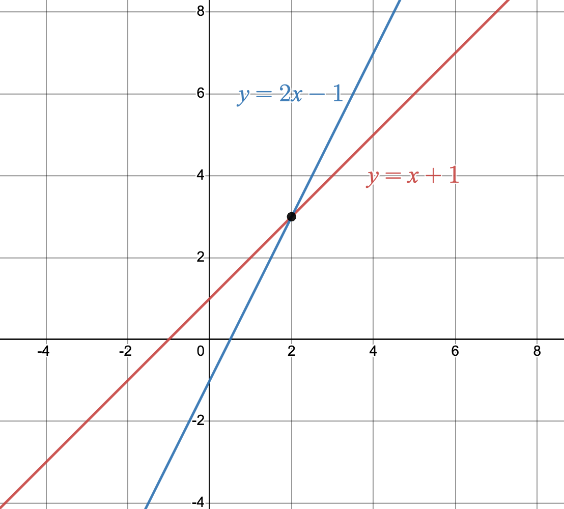
Example1.4.10.Solutions to Linear Equations Graphically.
In Example 1.4.9, we saw that a solution to the linear equation \(x+1 = 2x-1\) is \(x=2\text{.}\) Graphically, this means if we graphed \(y=x+1\) and \(y=2x-1\text{,}\) there would be an intersection point at \(x=2\text{:}\)
Activity1.4.4.
Give an example of a linear equation for each scenario below, or explain why an example does not exist. You are encouraged to think about each scenario graphically.
A linear equation which has exactly one solution.
A linear equation which has no solution.
A linear equation which has two solutions.
A linear equation in which every number is a solution.
Subsection1.4.4Summary
Question1.4.11.
What is the difference between a linear function and a proportional relationship?Answer.
A linear function is a function relationship which has a constant average rate of change between any two points. A proportional relationship is a specific type of linear function in which the \(y\)- intercept is equal to \(0\text{.}\)
Question1.4.12.
How is the equation of a linear function related to its graph?Answer.
The graph of a linear function can be determined by its slope and \(y\)-intercept. The slope determines whether the graph increases or decreases, and how quickly it increases or decreases. The \(y\)-intercept is a vertical shift of the graph of \(y=mx\) which determines where the graph crosses the \(y\)-axis.
Question1.4.13.
What do solutions to linear equations represent graphically?Answer.
Solutions to linear equations are points of intersection when graphing the lines on the left and right of the “\(=\)” sign. It is possible to have exactly one solution, no solution, or infinitely many solutions.
Exercises1.4.5Exercises
1.
Give an example, or explain why no example exists, of the graph of a function which is
linear but not proportional.
proportional but not linear.
linear and proportional.
2.
Write the equation of the line that passes through the points \((-2,10)\) and \((4,-3)\) using
point-slope form.
slope-intercept form.
3.
Find the solution(s) to \(mx+1 = 2x -3\text{,}\) where \(m\) is a parameter (your answer will be \(x=\) something in terms of \(m\)). For what value(s) of \(m\) is there no solution?
4.
Let \(p(x) =mx + p(0)\) be a linear function representing the price \(p(x)\) (in dollars) for riding \(x\) miles.