What is a mathematical model and why do we need them?
What are some common mathematical models?
What are some mathematical processes that can help us become better problem solvers?
A central theme in science is to study systems and how they change. Calculus can be viewed broadly as the study of change, and is therefore a useful tool to understand as a scientist. In this section we’ll begin to gain an understanding of the relationship between biology and mathematics. We begin with a warm-up describing a simple situation you may need to explore in the future.
Warm-Up1.1.1.
You are in the field measuring the height of a bine each day under certain conditions. You organize your measurements in the following table:
Table1.1.1.
\(t\) (days)
\(h\) (feet)
0
1
1
2.90
2
4.61
3
6.15
4
7.53
5
8.78
6
9.90
7
10.91
8
11.82
9
12.64
10
13.38
Organize your data as a graph.
What do you think the height of the bine will be after \(11\) days?
Subsection1.1.1Mathematical Models
If you compare your answer to Warm-Up 1.1.1 with other students, you will likely find that your estimation of the bine height after \(11\) days is different. You may have used slightly different reasoning to come up with your final answer.
Mathematical modeling is a way to convert data that we measure and observe into something that we can analyze and make predictions based on.
Mathematical Model.
A mathematical model is a mathematical representation that describes a system we have observed and measured.
The process of developing and using mathematical models often involves the following steps:
Observe and measure a system you are interested in.
Describe patterns in your observations and measurements.
Model the system with a mathematical representation that shares the patterns of the system.
Analyze the system and make predictions about the system using the mathematical model.
The focus of our text will be on analyzing and making predictions about how systems change given a mathematical model. The mathematical models we will use the most and will explore in much more detail are summarized below:
A function describes a specific type of relationships between different quantities. It can be expressed using multiple representations. Most models involve a function relationship.
A discrete-time dynamical system (DTDS) describes a sequence of measurements made at equally spaced intervals. Functions are an important component of these systems.
A continuous-time dynamical system (CTDS) describes measurements taken over an entire time interval. Functions are an important component of these systems.
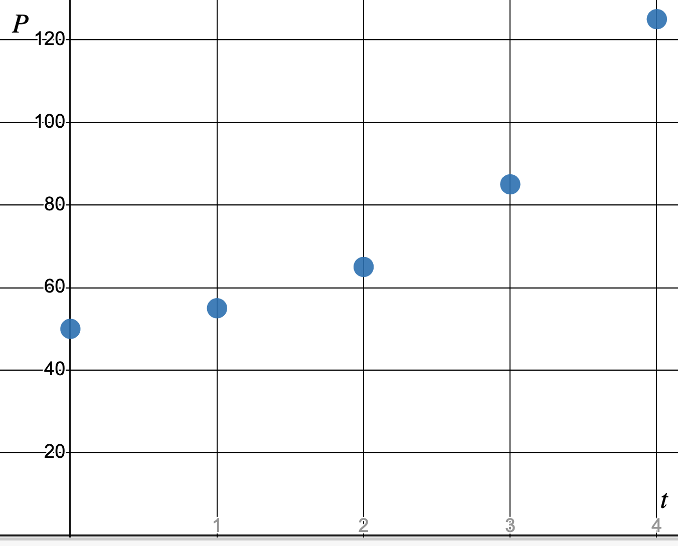
Example1.1.2.Discrete-Time Dynamical System.
Each year \(t\text{,}\) a population \(P\) of wolves is measured. A model which describes the population at a yearly interval is a discrete-time dynamical system. The graph of the relationship between population and time of such a model might look something like this:
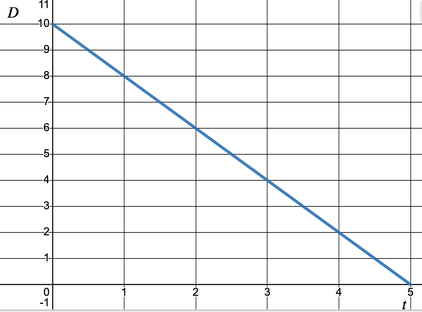
Example1.1.3.Continuous-Time Dynamical System.
As time \(t\) passes in seconds, my distance \(D\) from the door is measured. A model which describes my distance over the entire continuous time interval is a continuous-time dynamical system. The graph of the relationship between distance and time of such a model might look something like this:
In Example 1.1.2 and Example 1.1.3, we described the relationships explicitly; that is, we showed what a population value or a distance value would be for a given time value. In practice, this is not typically the representation we begin with for these models. For a DTDS, we give a first example below in Example 1.1.4, and will explore in much more detail in Section 1.7. The common representation and analysis of a CTDS is the main topic of Chapter 4.
Example1.1.4.Updating Function and Initial Value.
A strawberry plant begins as one plant. Each year, the plant produces \(2\) daughter plants. We can describe the growth of this system using an initial value (\(p_0\)) and an updating function, which uses the current population value (\(p_t\)) to describe what the next population value (\(p_{t+1}\)) will be:
Using the initial value and the updating function, we can determine the population of strawberry plants (\(p_t\)) at a given year \(t\text{:}\)
Table1.1.5.
\(t\)
\(p_t\)
0
\(p_0 =1\)
1
\(p_1 = p_0+2 =3\)
2
\(p_2 = p_1+2 = 5\)
3
\(p _3 = p_2+2 =7\)
Subsection1.1.2Mathematical Processes
Along with mathematical content, our text will also emphasize mathematical processes that enhance problem solving skills. The processes we will utilize most are:
Creating examples and counterexamples. We are likely used to watching an example from someone else to try and understand a concept, but the process of creating your own example or counterexample can be even more illuminating. In the process of constructing examples and counterexamples, you must think deeply about important aspects of a concept, and typically get repetition in applying relevant procedural tools. This process can be frustrating, as it does not usually happen quickly, but it can be a vital step in learning something well, and is a tools mathematicians use every day.
Utilizing technology. Technology can be an extremely useful tool for gaining intuition about a concept and for verifying conclusions. We’ll practice using technology in our study of Calculus to reinforce and enhance our conceptual understanding, not to replace it. The main tool we will use is Desmos 1 .
Activity1.1.2.Creating Examples.
Consider a population that changes according to the updating function
Find an example of an initial value \(b_0\) for which the population increases over time.
Find an example of an initial value \(b_0\) for which the population decreases over time.
Activity1.1.3.Utilizing Technology.
The following activity explores an algebra topic to practice utilizing technology to gain understanding of a topic. The general equation of a quadratic function is \(ax^2 + bx +c\text{.}\) Use the interactive below to answer the questions.
Which of \(a\text{,}\)\(b\text{,}\) or \(c\) determines whether the graph opens up or down?
What types of values make the graph open down?
Subsection1.1.3Summary
Below we re-visit the Motivating Questions from the beginning of the section. It is good practice to attempt to summarize in your own words before viewing the answers.
Question1.1.6.
What is a mathematical model and why do we need them?Answer.
A mathematical model is a mathematical representation that describes a system we have observed and measured. We can manipulate mathematical models in order to analyze and predict how a system is changing.
Common mathematical models are functions, discrete-time dynamical systems, and continuous-time dynamical systems.
Question1.1.8.
What are some mathematical processes that can help us become better problem solvers?Answer.
Processes that can help us become better problem solvers are creating examples and counterexamples, and learning how to utilize technology in a way that reinforces and enhances our understanding of a concept.
Exercises1.1.4Exercises
1.
Use the Desmos graphing calculator 2 to plot the points given in the table of Warm-Up 1.1.1. Then graph \(y = -19 \cdot 0.9^x + 20\text{.}\) What do you notice? Use this graph to predict the height of the bine after \(11\) days.
2.
The representations of models that we will practice working with in this text are motivated by the models that are used to analyze real systems.
Browse the following papers which describe research in the field of biology. Focus on the models being used and how they are represented.
Reflect on your observations by considering the following questions:
What types of models do you see?
What do you notice about the use of numbers in the models?
What are some questions that you have about how symbols are being used in the models? The way symbols are used to create meaning is called notation, and we will address many questions regarding notation as we continue our development and analysis of mathematical models.