Thermal convection

In collaboration with geoscientists, I have a research program that involves simulating thermal convection in the Earth mantle. The equations that describe these processes are generalizations of the Boussinesq equations.

Some pictures and movies from my early attempts can be found as part of the step-31 and step-32 tutorial programs of deal.II. More recent results come from our open source mantle convection code Aspect:

More movies can be found at the ASPECT picture gallery.

Optical tomography

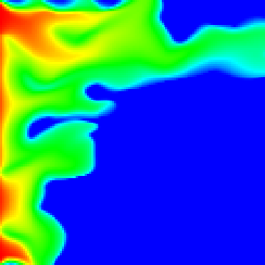
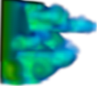
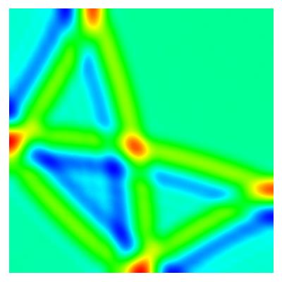
These are a few pictures of simulations of optical tomography in a geometry that corresponds to a breast cancer phantom used in some of our studies.

The pictures correspond to how we simulated light propagation in the breast phantom: an incident laser illuminates a small region on the surface of the skin; in the top pictures this is a strip at the left, in the bottom left picture a strip to the right. The light diffuses into the tissue, as shown by the isocontours emanating from this area.

The incident light is absorbed by regular tissue as well as a fluorescent dye that is injected and that is specific to tumor cells. The dye then re-emits light at a different wave length that we then detect; the intensity of this fluorescent light is shown in the first three images by the isosurfaces centered at the tumor at the middle of the domain.

The bottom right image shows the result of re-constructing the dye concentration, and thereby the tumor location, from the measured fluorescent light intensities. It shows a tumor at the center of the domain.

Absorbing boundary conditions

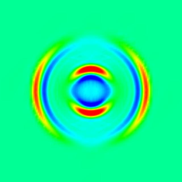
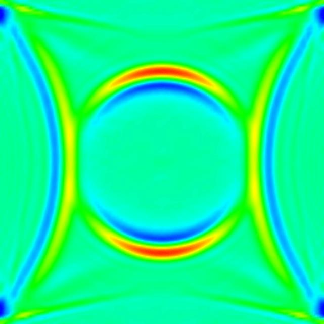
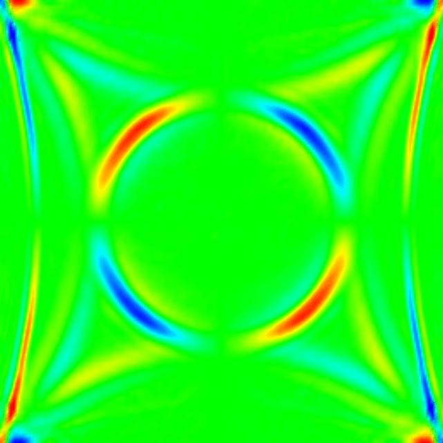
In many situations, one would like to simulate wave propagation phenomena in unbounded regions. For example, consider a sound source right next to a sphere and you want to place a microphone on the other side of the sphere. Then, you will usually not be interested in the main part of the sound signal that travels to everywhere except to the microphone. Worse even, compared to the dimensions of the sphere, the region of air around it is usually quite large, and we would have to use much of our numerical efforts to compute how the sound signal propagates in these vast regions in which we are not interested at all.

One way out of this problem is to restrict the domain on which we compute our solution to a region around the sphere, and doing so in such a way that we know that no signal that has ever left this region can influence the signals we measure with the microphone. Thus, we introduce an artificial boundary (as opposed to a physical one, since we introduce a boundary into the extending region of air around our ensemble of sound source, sphere, and microphone), and for a numerical approximation of the problem at hand, we have to pose conditions on this boundary that describe a boundary through which all waves can travel unhindered, but from which no waves can come back.

Posing such boundary conditions is not simple for more than one space dimension. A common approximation is the first order condition by Bayliss and Turkell (or Engquist and Majda), but it is not the exact boundary condition and generates spurious reflections. These can be seen in the pictures above: the dark blue wave in the second picture is a spurious reflection of the original wave at the outer boundary, while the physical reflection of the initial wave from the sphere in the center can clearly be seen. As time proceeds the initial wave travels forth, and is diffracted from the sphere, as can be seen in pictures 4-6. In the last picture, the original wave has left the domain and only that part that was diffracted can be seen, where the two parts coming right and left around the sphere presently meet at its bottom. However, the blue spurious reflection from the beginning travels all along and is more intense in the last picture even than the diffracted part of the original wave. (Note that the scales of the pictures vary, so that the spurious wave does not gain in intensity during time, only the extreme colors move to lower amplitudes of the waves. Please also excuse the missing pieces at the left and right edges - I have no clue what is going on here, in any case the program is computing with a spherical outer boundary.)

Approximate absorbing boundary conditions

Movie (2.0MB)

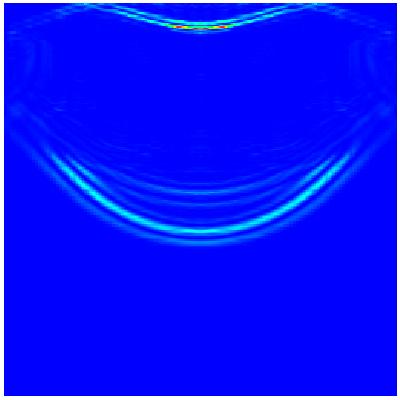
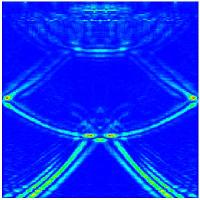
Sometimes, it is not necessary to go to some lengths in inventing exactly absorbing boundary conditions, but approximate ones are sufficient. The pictures above and the movie shows an example of such a boundary condition in action. The domain here is thought to represent the earth crust, from the surface down to the Moho discontinuity at a depth of 30 km. It is (very crudely) approximated by three layers, one low density low wave speed layer at the top of 3 km depth, a high density high wave speed layer between 3 and 6 km depth, and below that a layer of medium density and medium wave speed. No attenuation is included in the model. Then a source is placed into the middle layer and we track how the waves travel outwards (the reflecting vertical sides are unphysical, so please ignore them) and eventually hits the lower boundary. The Moho discontinuity is usually considered an absorbing boundary, so we here simulate it by a simple first order absorbing boundary condition. You can readily see that the waves in the pictures and movie are absorbed without noticable reflections there.

Just for comparison, we show a comparable movie with reflecting boundary conditions at the bottom. For this movie, the source wave length was also chosen three times smaller than for the other example, increasing the necessary numerical work by approximately a factor or 30. Click here for this second movie (2.0MB). It is obvious that the waves are reflected back from the bottom, which however is nonphysical behaviour.

Multiphase flow

Assume we wanted to model how a mixture of water and oil flows in an oil reservoir. This is a practically relevant question, since oil reservoirs are often produced by pumping in water through one well, which is then pushed towards another well that pumps the resulting mixture out to the surface. In addition, oil reservoirs are often heterogenous due to cracks and weakness in the rocks, so the fluid does not flow along a nicely defined front, but in shapes that are called "fingers". The following two images clearly show this phenomenon, in both 2d and 3d simulations:

Movie (1.5MB)	Movie (1.6MB)

By clicking on the text below each of these pictures, you can get a short movie that shows the evolution of the water saturation in these simulations.

The simulations shown here were done with the help of the deal.II library, of which I am the main author. In particular, the program that computes these images is the step-21 tutorial program that is part of the publicly available distribution of this library.

Elastic Waves

Movie (3.8MB)	Movie (3.8MB)

These pictures are from a simulation of the elastic wave equation. This equation describes the displacement of the particles within an elastic body in each of the coordinate directions.

Click on the text "Movie" below the pictures to see the waves travelling!

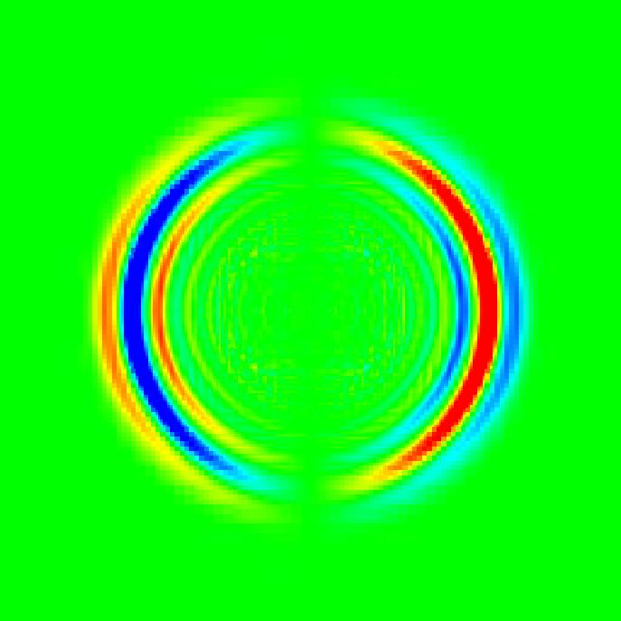
Here, we initially displaced a particle (or better a whole region) at the center of the body a little bit to the right and let it snap back then. To the left, the displacement in x-direction is shown at two subsequent times, to the right is the displacement in vertical direction. The fast pressure waves (P waves) travelling to the left and right can clearly be distinguished from the slow shear waves (S waves) travelling vertically.

P and S waves can be easily visualized by plotting the divergence and curl of the wave field. The first is the P wave and the latter the S wave. Below are two pictures showing these components (at the same time - note the difference in diameter of the waves), and the movies also nicely show conversion of P to S waves: when the P waves hit the left and right boundaries, S waves suddenly appear where there have been none before! (Note that for the simulations below, the S wave velocity has been set differently to the one for the simulations above; also, we have only computed the divergence and curl once per cell, which makes the output look a bit `blocky'.)

Movie (3.8MB)	Movie (3.8MB)

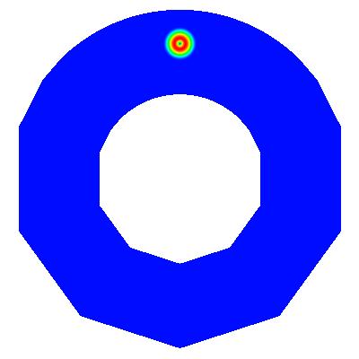
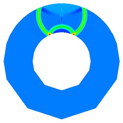
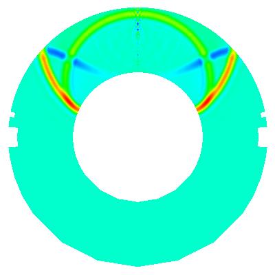
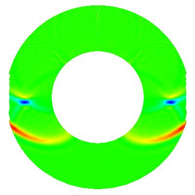
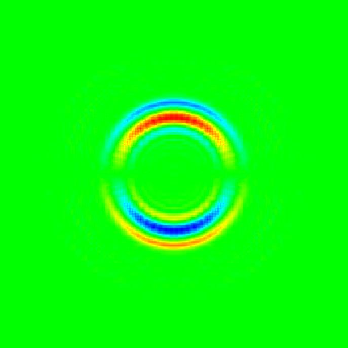
Surface waves at curved boundaries

Click here for a movie (5MB)

This is a toy simulation of wave propagation in a ring domain. However, there is still some content in it since one can so clearly see that the waves travelling around the ring form surface waves. This is also what usually happens with earthquake waves!

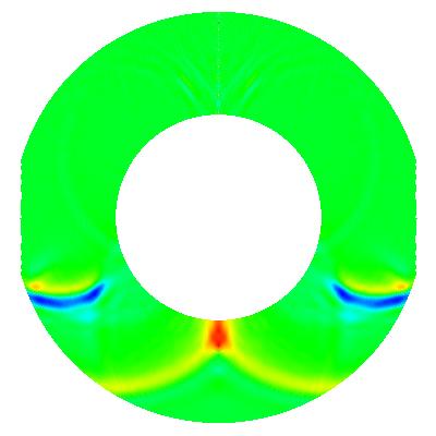
Below is another simulation, with a different source and a smaller ring.

(Please note: the two movies above and below have a size that not all mpeg-players understand. While you can view these movies on most Unix systems, you mileage may vary on other systems.)

Click here for a movie (4MB)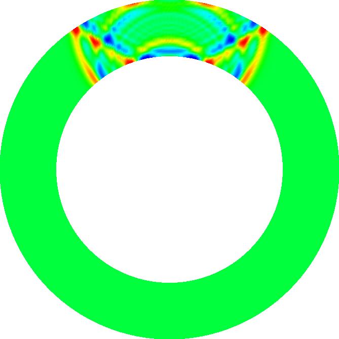

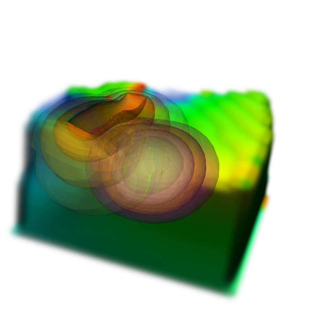
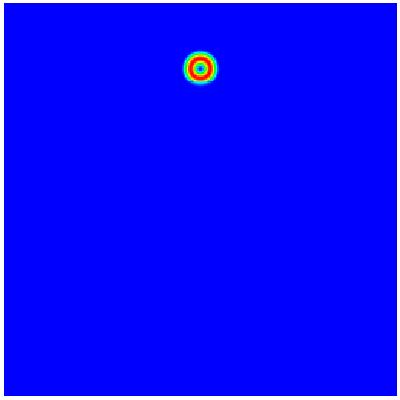
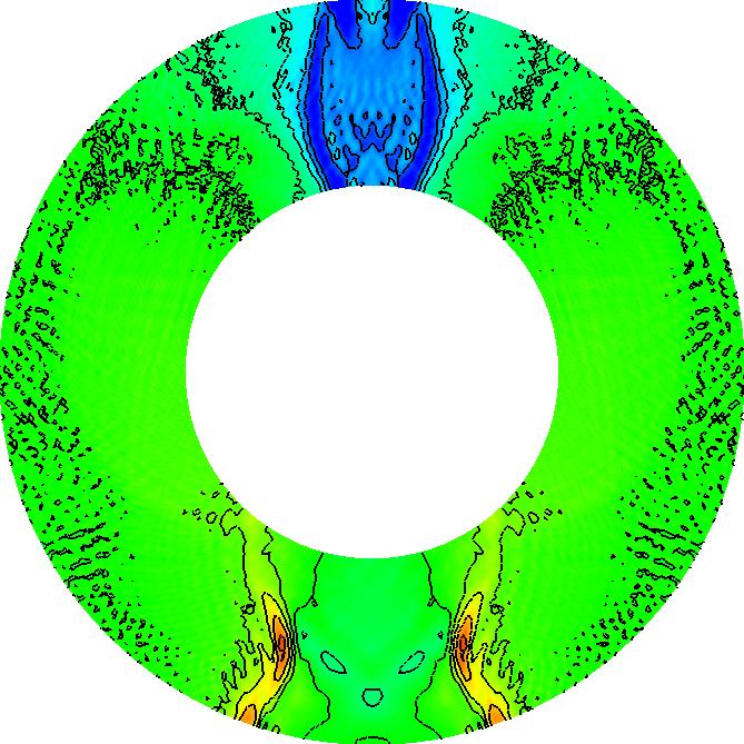
Acoustic waves in a cylindrical coordinate system

The following picture and movie are from a simulation in a cylindrical coordinate system:

Click here for a movie (3.1MB)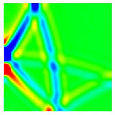

Cylindrical coordinates are used to simulate three dimensional wave motion in a two dimensional space when the domain and the wave field have rotational symmetry around an axis. In the picture above, this axis was the left side of the square.

Computations were performed on a rather coarse grid, of which you can see effects at some time steps, but the main features can be gathered, I believe.

There is one important thing that can be seen: behind the main wave (i.e. the positive and negative amplitudes colored in red and blue), there is nothing. This is a particular feature of three dimensional wave propagation, where mathematically speaking Greens's function is a measure one a ball around the origin. In more understandable words: if someone shouts at you, you will hear him after a small time which the sound takes to get to you, but then there is silence.

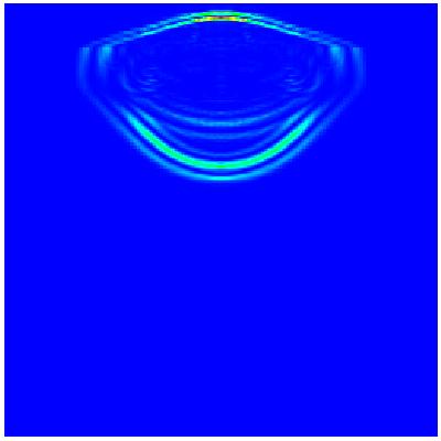
In a two dimensional world things are different. If you imagine what happens when you throw a stone into the water, you remember that there is an infinite series of waves coming out of the spot where the stone hit the water surface. These waves are getting continuously smaller, but the main thing to note is that after the front wave, there are others following.

It is difficult to show this effect in a movie since the waves are getting smaller quickly and the smaller ones will not be visible. We therefore show only a movie in a similar configuration as the one above, but in a truly two dimensional domain.

Click here for a movie (3.1MB)

The lack of silence after the first wave has arrived means that if we were living in a two dimensional world, there would be a reverberation after each sound. People would say something, then shut their mouth, but there would still be coming a sound from their direction. It has been said that it would be very loud in a two dimensional world...