Combinatorics
BlueBox
Enumeration and Structure
Course Notes – MATH 501/2
![[Uncaptioned image]](x147.png)
LaTeX-ed on August 25, 2025
Alexander Hulpke
Department of Mathematics
Colorado State University
1874 Campus Delivery
Fort Collins, CO, 80523
{epigraphs}
\qitemTitle graphics:
Window in the Southern Transept of the Cathedral in Cologne (detail)
Gerhard Richter
These notes are accompanying my course MATH 501/2, Combinatorics,
held Fall 2025 at Colorado State University.
©2025 Alexander Hulpke. Copying for personal use is permitted.
1 Preface
Counting is innate to man.
History of India
Abū Rayhān Muhammad ibn Ahmad Al-Bīrūnī
This are lecture notes I prepared for a graduate Combinatorics course which ran in 2016/17, 2020/21, 2024 and 2025 at Colorado State University.
They started many years ago from an attempt to supplement the book [cameron] (which has great taste in selecting topics, but sometimes is exceedingly terse) with further explanations and topics, without aiming for the encyclopedic completeness of [stanley1, stanley2].
In compiling these notes, In addition to the books already mentioned, I have benefitted from: [cameron, cameronlint, godsilroyle, lidlniederreiterapp, lintwilson, hall, concrete, knuth3, reichmeider].
You are welcome to use these notes freely for your own courses or students – I’d be indebted to hear if you found them useful.
Fort Collins, \thedate
Alexander Hulpke
hulpke@colostate.edu
Chapter 0 Introduction
A
combinatorial structure is one which has combinatorial properties.
Combinatorial properties are those possessed by combinatorial structures. So
formal definitions are not getting us anywhere.
We shall leave combinatorial structure as an undefined term. […]Course on Undergraduate Combinatorics
Solomon Golomb and Andy Liu
1 What is Combinatorics?
If one looks at university mathematics classes around 1920, one already finds the basic pattern of many current courses. Single-variable analysis had already taken much of its present shape. Algebra had begun to formalize groups, rings, and fields — concepts that, a few years later, looked very much like what is taught today. Much of the theory of differential equations was known, and numerical methods lacked only the availability of fast computers. But there was little combinatorics beyond the basic counting formulas used in statistics. Combinatorics began to grow suddenly in the 1950s and 1960s, in part motivated by the advent of computers, and arguably did not have a standard list of topics until the 1980s or 1990s. It differs from many other areas of mathematics in that it was not driven by a small number of deep (often unresolved) problems, but by the observation that problems from seemingly different areas actually follow similar patterns and can be studied with similar methods. Its scope, in the broadest sense, is the study of the different ways objects can be related to one another.
This investigation naturally splits into three parts: The question of existence (Can certain configurations exist?) Counting the number of possible configurations. (If we can count them it often implies we have a good overview over what can exist.) And finding extreme, often optimal, cases.
This course looks at combinatorics split into two main areas, roughly corresponding to semesters: the first is enumerative combinatorics, the study of counting the different ways configurations can be set up. The second is the study of properties of combinatorial structures that consists of many objects subject to certain prescribed conditions.
2 Prerequisites
This being a graduate class we shall assume knowledge of some topics that have been covered in undergraduate classes. In particular we shall use:
Sets, Functions, Relations
We assume the reader is comfortable with the concept of sets and standard constructs such as Cartesian products. We denote the set of all subsets of by , it is called the power set of .
A relation on a set is a subset of , functions can be considered as a particular class of relations. We thus might consider a function as a subset of .
Another important class of relations are equivalence relations. Via equivalence classes they correspond to partitions of the set.
Induction
The technique of proof by induction is intimately related to the concept of recursion. It is assumed, that the reader is comfortable with the various variants (different starting values, referring to multiple previous values, postulating a smallest counterexample) of finite induction. We also might sometimes just state that a proof follows by induction, if base case or inductive step are obvious or standard.
1 Abstract Algebra
Abstract algebra is often useful in providing a formal framework for describing objects. We assume the reader is familiar with the standard concepts from an undergraduate abstract algebra class – groups, permutations (we multiply permutations from left to right), cycle form, polynomial rings, finite fields, and linear algebra.
2 Graph Terminology
This being a graduate class, the assumption is that the reader has encountered the basic definitions of graph theory – such as: vertex, edge, degree, directed/undirected, path, tree – already in an undergraduate class.
3 Calculus
It often comes as a surprise to students , that combinatorics – this epitome of discrete mathematics – uses techniques from calculus. Some of it is the classical use of approximations to estimate growth, but we shall also need it as a toolset for manipulating power series. Still, there is no need for the reader to worry that we would encounter messy approximations, convergence tests, or bathtubs that are filled while simultaneously draining.
3 OEIS
A problem that arises often in combinatorics is that we can easily describe small examples, but that it is initially hard to see the underlying patterns. For example, we might be able to count the total number of objects of small size, but will be unable to count how many there are of larger size. In investigating such situations, the Online Encyclopedia of Integer Sequences (OEIS, at oeis.org) is an invaluable tool that allows to look up number sequences that fit the particular pattern Given by a few values , and for many of these gives a huge number of connections and references . Sequences in this encyclopedia have a “storage number” starting with the letter ”A”, and we will refer to these at times by an indicator box OEIS A002106.
Chapter 1 Basic Counting
One of the basic tasks of combinatorics is to determine the cardinality of (finite) classes of objects. Beyond basic applicability of such a number – for example to estimate probabilities – the actual process of counting may be of interest, as it gives further insight into the problem:
-
•
If we cannot count a class of objects, we cannot claim that we know it.
-
•
The process of enumeration might – for example by giving a bijection between classes of different sets – uncover a relation between different classes of objects.
-
•
The process of counting might lend itself to become constructive, that is allow an actual construction of (or iteration through) all objects in the class.
The class of objects might have a clear mathematical description – e.g., all subsets of the set . In other situations the description itself needs to be translated into proper mathematical language. For example:
Definition 1 (Derangements, informal definition).
Given letters and addressed envelopes, a derangement is an assignment of letters to envelopes such that no letter is in the correct envelope.
(How many derangement of exist? This particular problem will be solved in section 5.)
Here the translation to more formal objects is that we consider the letters and envelopes to be numbered from to , and the assignment being a function. That is:
Definition 2 (Derangements).
For an integer , a derangement is a bijection on (i.e. a permutation), such that for all .
We will start in this chapter by considering the enumeration of some basic constructs – sets and sequences. More interesting problems, such as the derangements here, arise later if further conditions restrict to sub-classes, or if obvious descriptions could have multiple sequences describe the same object.
1 Basic Counting of Sequences and Sets
I am the sea of permutation.
I live beyond interpretation.
I scramble all the names and the combinations.
I penetrate the walls of explanation.
Lay My Love
Brian Eno
The number of elements of a set , denoted by (or sometimes as ) and called its cardinality, is defined111We only deal with the finite case here, there are generalizations for infinite sets as the unique , such that there is a bijective function from to .
There are three basic principles that underlie counting:
- Disjoint Union
-
If with , then .
- Cartesian product
-
.
- Equivalence classes
-
If we can represent each element of in different ways by elements of , then .
A sequence (or tuple) of length is simply an element of the -fold cartesian product. Entries are chosen independently, that is if the first entry has choices and the second entry , there are possible choices for a length two sequence. Thus, if we consider sequences of length , entries chosen from a set of cardinality , there are such sequences.
This allows for duplication of entries, but in some cases – arranging objects in sequence – this is not desired. In this case we can still choose entries in the first position, but in the second position need to avoid the entry already chosen in the first position, giving options. (The number of options is always the same, the actual set of options of course depends on the choice in the first position.) The number of sequences of length thus is , called222Warning: The notation has different meaning in other areas of mathematics! “ lower factorial ”.
This could be continued up to a sequence of length (after which all element choices have been exhausted). Such a sequence is called a permutation of . There are such permutations.
Next we consider sets of elements. While every duplicate-free sequence describes a set, sequences that have the same elements arranged in different order describe the same set. Every set of elements from thus will be described by different duplicate-free sequences. To enumerate sets, we therefore need to divide by this factor, and get for the number of -element sets from the count given by the binomial coefficient
Note (using a convention of ) we get that . It also can be convenient to define for or .
Often one counting process can be modified to count somewhat different objects: Consider compositions of a number into parts, that is ways of writing as a sum of exactly positive integers with ordering being relevant. For example are the 3 possible compositions of into parts.
To get a formula of the number of possibilities, write the maximum composition
which has plus-signs. We obtain the possible compositions into parts by grouping summands together to only have summands. That is, we designate plus signs from the given possible ones as giving us the separation. The number of possibilities thus is .
If we also want to allow summands of when writing as a sum of terms, we can simply assume that we temporarily add to each summand. This guarantees that each summand is positive, but adds to the sum. We thus count the number of ways to express as a sum of summands which is by the previous formula .
Check this for and .
Again, slightly rephrasing the problem, this is also the number of multisets, that is set-like collections in which we allow the same element to appear multiple times, with elements chosen from possibilities, the -th summand indicating how often the -th element is chosen.
Swapping the role of and , We denote by (the second equality follows from Prop.4 a) the number of -element multisets chosen from possibilities.
The results of the previous paragraphs are summarized in the following theorem:
Theorem 3.
The number of ways to select objects from a set of is given by the following table:
| Repetition | No Repetition | |
|---|---|---|
| Order significant | ||
| (sequences) | ||
| Order not significant | ||
| (sets) |
Note 1.1.
Instead of using the word significant some books talk about ordered or unordered sequences. I find this confusing, as the use of ordered is opposite that of the word sorted which has the same meaning in common language. We therefore use the language of significant.
2 Bijections and Double Counting
As long as there is no double counting, Section 3(a) adopts the principle of
the recent cases allowing recovery of both a complainants actual losses and
a misappropriator’s unjust benefit…
Draft of Uniform Trade Secrets Act
American Bar Association
In this section we consider two further important counting principles that can be used to build on the basic constructs.
Instead of counting a set of objects directly, it might be easiest to establish a bijection to another set , that is a function which is one-to-one (also called injective) and onto (also called surjective). Once such a function has been established we know that and if we know we thus have counted .
We used this idea already above when we were counting compositions by instead considering possible positions of plus signs.
As a further example, consider the following problem: We have an grid of points with horizontal and vertical connections (depicted in figure 1 for ) and want to count the number of different paths from the bottom left, to the top right corner, that only go right or up.
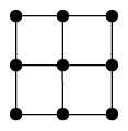
Each such path thus has exactly right steps, and up steps. We thus (this already could be considered as one bijection) could count instead sequences ( is right, is up) of length that contain exactly ones (and zeros). Denote the set of such sequences by .
To determine , we observe that each sequence is determined uniquely by the positions of the ones and there are exactly of them. Thus let be the set of all -element subsets of .
We define to assign to a sequence the positions of the ones, .
As every sequence has exactly ones, indeed goes from to . As the positions of the ones define the sequence, is injective. And as we clearly can construct a sequence which has ones in exactly given positions, is surjective as well. Thus is a bijection.
We know that , this is also the cardinality of .
Check this for , .
The second useful technique is to “double counting”, counting the same set in two different ways (which is a bijection from a set to itself). Both counts must give the same result, which can often give rise to interesting identities. The following lemma is an example of this paradigm:
Lemma 2.1 (Handshaking Lemma).
At a convention (where not everyone greets everyone else but no pair greets twice), the number of delegates who shake hands an odd number of times is even.
Proof 2.2.
we assume without loss of generality that the delegates are . Consider the set of handshakes
We know that if is in , so is . This means that is even, where is the total number of handshakes occurring.
On the other hand, let be the number of pairs with in the first position. We thus get . If a sum of numbers is even, there must be an even number of odd summands.
But is also the number of times that shakes hands, proving the result.
About binomial theorem I’m teeming with a lot o’ news,
With many cheerful facts about the square of the hypotenuse.
The Pirates of Penzance
W.S. Gilbert
The combinatorial interpretation of binomial coefficients and double counting allows us to easily prove some identities for binomial coefficients (which typically are proven by induction in undergraduate classes):
Proposition 4.
Let be nonnegative integers with . Then:
-
a)
.
-
b)
.
-
c)
(Pascal’s triangle).
-
d)
.
-
e)
.
-
f)
(Binomial Theorem).
Proof 2.3.
a) Instead of selecting a subset of elements we could select the
elements not in the set.
b) Suppose we want to count committees of people (out of ) with a
designated chair. We can do so by either choosing first the
committees and then for each team the possible chairs out of the committee
members. Or we choose first
the possible chairs and then the remaining committee members out of
the remaining persons.
c) Suppose that I am part of a group that contains persons
and we want to determine subsets of this group that contain people. These
either include me
(and further persons from the others), or do not
include me and thus from the other people.
d) We count the total number of subsets of a set with elements.
Each subset can be described by a sequence of length , indicating
whether the -th element is in the set.
e) Suppose we have men and women and we want to select groups of
persons. This is the right hand side.
The number of possibilities with
exactly women is by a).
The left hand of the equation simply sums these over all possible .
f) Clearly is a polynomial of degree . The coefficient for
gives the number of possibilities to choose the -summand when multiplying
out the product
of factors so that there are such summands overall. This is simply the number of -subsets, .
Prove the theorem using induction. Compare the effort. Which method gives you more insight?
3 Stirling’s Estimate
Since the factorial function is somewhat unhandy in estimates, it can be useful to have an approximation in terms of elementary functions. The most prominent of such estimates is given by Stirling’s formula. Our description follows [fellerstirling]:
Theorem 5.
| (1) |
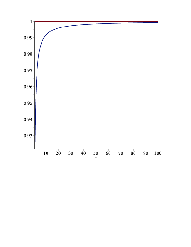
Here means that the quotient of the estimate and the true value is bounded by , that is the relative error is . Figure 2 shows a plot of the ratio of the estimate to .
Proof 3.1.
Consider the natural333all logarithms in this book are natural, unless stated differently logarithm of the factorial:
If we define a step function , we thus have that is an integral of . We also know that
We thus need to consider the integral over . To avoid divergence issues, we consider this in two parts. Let
and
Then
A substitution gives
from which we see that . By the Leibniz’ criterion thus converges to a value and we have that
Taking the exponential function we get that
with .
Using standard analysis techniques, one can now show that ; see [fellerstirling] for details. Alternatively, in concrete calculations, we could simply approximate the value to any accuracy desired.
The appearance of might seem surprising, but the following example shows that it arises naturally in this context:
Proposition 6.
The number of all sequences (of arbitrary length) without repetition that can be formed from objects is .
We note that no sequence can have length more than , as this would require repetition.
Proof 3.2.
If we have a sequence of length , there are sequences of length . Summing over all values of we get (with an index shift, replacing by ):
Using the Taylor series for we see that
This is an example (if we ignore language meaning) of the popular problem how many words could be formed from the letters of a given word, if no letters are duplicate.
If we allow duplicate letters the situation gets harder. For example, consider words (ignoring meaning) made from the letters of the word COLORADO. The letter O occurs thrice, the other five letters only once. If a word contains at most one O, the formula from above gives such words.
For more than one O, the above formula can’t be used any longer, but we need to go back to summations. If the word contains two O, and other letters there are options to select these letters and possibility to arrange the letters (the denominator 2 making up for the fact that both O cannot be distinguished). Thus we get
such words.
If the word contains three O, and other letters we get a similar formula, but with a cofactor , reflecting the arrangements of the three O which yield the same word. We thus have
possibilities, summing up to possibilities in total.
Lucky we do not live in MISSISSIPPI!
4 The Twelvefold Way
A generalization of counting sets and sequences is given by considering functions between finite sets. We shall consider functions with and . These functions could be arbitrary, injective, or surjective.
What does the concept of order (in)significant mean in this context? If the order is not significant, we actually only care about the set of values of a function, but not the values on particular elements. That is, all the elements of are equivalent, we call them indistinguishable or unlabeled (since labels will force objects to be different). Otherwise we talk about distinguishable or labeled objects.
Formally, we are counting equivalence classes of functions, in which two functions are called -equivalent, if there is a bijection such that for all .
Similarly, we define an -equivalence of function, calling s and equivalent, if there is such that for all . If we say the elements of are indistinguishable, we count functions up to -equivalence.
We can combine both equivalences to get even larger equivalence classes, which are the case of elements of both and being indistinguishable.
(The reader might feel this to be insufficiently stringent, or wonder about the case of different classes of equivalent objects. We will treat such situations in Section LABEL:polya under the framework of group actions.)
This setup ( and distinguishable or not and functions being injective, surjective or neither) gives in total possible classes of functions. This set of counting problems is called the Twelvefold Way in [stanley1, Section 1.9] (and attributed there to Gian-Carlo Rota).
For each of the 12 categories, give an example of a concrete counting problem in common language. Say, we have balls and boxes (either of them might be labeled), and we might require that no box has more than one ball, or that every box contains at least one ball.
Say, we have and . Then we have the following functions :
- All functions:
-
There are 9 functions, namely (giving functions as sequences of values):
- Injective functions:
-
There are 6 functions, namely
- Surjective functions:
-
There are no such functions, but there are 6 functions from to , namely:
- Up to permutation of
-
So we consider only the sets of values, which gives 6 possibilities:
- Injective, up to permutation of
-
The values need to be different, so 3 possibilities:
- Surjective, up to permutation of
-
There are no such functions, but there are 2 such functions from to , namely:
- Up to permutations of
-
Since , the question is just whether the two values are the same or not:
- Injective, up to permutations of
-
Here is the only such function.
- Surjective, up to permutations of
-
Again, no such function, but from to there are 3 such functions namely
- Up to permutations of and
-
Again two possibilities, but if , there are three possibilities, namely
- Injective, up to permutations of and
-
Again, is the only such function.
- Surjective, up to permutations of and
-
Again, no such function, but from to there is one, namely .
We are now getting ready to give formulas for the number of functions in each class, depending only on and . For this we introduce the following definitions. Determining closed formulae for these is not always easy, and will require further work in subsequent chapters.
A partition of a set is a collection of subsets (called parts or cells) such that for all :
-
•
-
•
for .
Note that a partition of a set gives an equivalence relation and that any equivalence relation on a set defines a partition into equivalence classes.
Definition 7.
We denote the number of partitions of into (non-empty) parts by . It is called the Stirling number of the second kind444There also is a Stirling number of the first kind OEIS A0082h7. The total number of partitions of is given by the Bell number OEIS A000110
There are partitions of the set .
Again we might want to set unless .
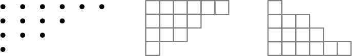
In some cases we shall care not which numbers are in which cells of a partition, but only the size of the cells. (That is, we only care about writing as a sum over an increasing sequence of positive integers: .) Sometimes this is called an integer partition, a Young diagram, or a Ferrers diagram555The difference between the last two is purely in whether we draw boxes or circles.. Figure 3 shows these diagrams for partition . In one style (called ”English”), the length of rows decrease as one goes downwards, in another (”French”) they do as one goes upwards.
We denote the number of partitions of into parts (ignoring which numbers are in which part) by , the total number of partitions by . OEIS A000041.
Again we study the function later, however here we shall not achieve a closed formula for the value.
We have , but . This is because the three partitions , , all have the same cell size pattern.
1 The twelvefold way theorem
We now extend the table of theorem 3:
Theorem 8.
if are finite sets with and , the number of (equivalence classes of) functions is given by the following table. (In the first two columns, d/i indicates whether elements are considered distinguishable or indistinguishable. The boxed numbers refer to the explanations in the proof.):
| arbitrary | injective | surjective | ||
|---|---|---|---|---|
| d | d | |||
| i | d | |||
| d | i | |||
| i | i |
Proof 4.1.
If is distinguishable, we can simply write the elements of in a row and consider a function on as a sequence of values. In 1), we thus have sequences of length with possible values, in 2) such sequences without repetition, both formulas we already know.
If such a sequence takes exactly values, each value can be taken to indicate the cell of a partition into parts, into which is placed. As we consider a partition as a set of parts, it does not distinguish the elements of , that shows that the value in 9) has to be . If we distinguish the elements of we need to account for the possible arrangements of cells, yielding the value in 3).
Similarly to 9), if we do not require to be surjective, the number of different values of gives us the number of parts. Up to different parts are possible, thus we need to add the values of the Stirling numbers.
To get 12) from 9) and 10) from 7) we notice that making the elements of indistinguishable simply means that we only care about the sizes of the parts, not which number is in which part. This means that the Stirling number gets replaced by the partition (shape) count .
If we again start at 1) but now consider the elements of as indistinguishable, we go from sequences to sets. If is injective we have ordinary sets, in the general case multisets, and have already established the results of 4) and 5).
For 6), we interpret the distinct values of to separate the elements of into parts. This is a composition of into parts, for which the count has been established.
In 8) and 11), finally, injectivity demands that we assign all elements of to different values which is only possible if . As we do not distinguish the elements of it does not matter what the actual values are, thus there is only one such function up to equivalence.
Chapter 2 Recurrence and Generating Functions
There’s al-gebra. That’s like sums with letters.
For…for people whose brains aren’t clever enough for numbers, see?
Jingo
Terry Pratchett
Finding a closed formula for a combinatorial counting function can be hard. It often is much easier to establish a recursion, based on a reduction of the problem. Such a reduction often is the principal tool when constructing all objects in the respective class.
An easy example of such a situation is given by the number of partitions of , given by the Bell numbers :
Lemma 0.1.
For we have:
Proof 0.2.
Consider a partition of . Being a partition, it must have in one cell. We group the partitions according to how many points are in the cell containing . If there are elements in this cell, there are options for the other points in this cell. And the rest of the partition is simply a partition of the remaining points.
1 Power Series – A touch of Calculus
A powerful technique for working with recurrence relations is that of generating functions. The definition is easy, for a counting function defined on the nonnegative integers we define the associated generating function as the power series
Here is the ring of formal power series in , that is the set of all formal sums with .
When writing down such objects, we ignore the question whether the series converges, i.e. whether can be interpreted as a function on a subset of the real numbers.
The reader interested in a rigorous, self-contained, presentation of the theory of formal power series, that does not require any reliance of results from analysis, can find it in [sambale2024].
Addition and multiplication are as one would expect: If and we define new power series and by:
With this arithmetic becomes a commutative ring. (There is no convergence issue, as the sum over is always finite.)
We also define two operators, called differentiation and integration on by
and
(with the integration constant is set as ).
Two power series are equal if and only if all coefficients are equal. An identity involving a power series as a variable is called a functional equation.
As a “shorthand”, pretending we knew nothing from Calculus (after all, we do not establish convergence), we define the following names for particular power series:
and note111All of this can either be proven directly for power series; alternatively, we choose in the interval of convergence, use results from Calculus, and obtain the result from the uniqueness of power series representations. that the usual functional identities , , and differential identities , hold.
A telescoping argument shows that for we have that , that is we can use the geometric series identity
to embed rational functions (whose denominators factor completely; this can be taken as given if we allow for complex coefficients) into the ring of power series.
For a real number , we define222Unless is an integer, this is a definition in the ring of formal power series. the generalized binomial coefficient as:
as well as a series representation of the -th power:
For obvious reasons we call this definition the binomial formula. Note that for integral this agrees with the usual definition of exponents and binomial coefficients, so there is no conflict with the traditional definition of exponents.
We also notice that for arbitrary we have that and .
Up to this point, generating functions seem to be a formality for formalities sake. They however come into their own with the following observations: Operations on the entries of a sequence, relations amongst its entries (such as recursion), or a sequence having been built on top of other sequences often have natural analogues with generating functions. Recursive identities amongst a coefficient sequence then become functional equations or differential equations for the generating functions.
If these equations have solutions, known start values typically give uniqueness of the solution, and (assuming it converges in an open interval), its power series representation must be identical to the generating function. Methods from Analysis, such as Taylor’s theorem, then can be used to determine expressions for the terms of the sequence.
Before describing this more formally, let us look at a toy example:
We define a function recursively by setting and . (This recursion comes from the number of subsets of a set of cardinality – fix one element and distinguish between subsets containing this element and those that don’t.) The associated generating function is . We now observe that
We solve this functional equation as
and (geometric series!) obtain the power series representation
this allows us to conclude that , solving the recursion (and giving the combinatorial result (which we knew already by another method) that a set of cardinality has subsets.)
1 Operations on Generating Functions
To prepare us for working with generating functions, let’s look in more detail on what generating function operations do with the coefficients.
For this, assume that and are sequences, associated to generating functions and , respectively.
We start with basic linearity. is the generating function associated to the sequence . The case is sometimes called the sum rule, describing the case that and count the cardinality of disjoint sets and the cardinality of their unions.
Shifting
Shifting the indices corresponds to multiplication by (positive or negative) powers of .
Differentiation
If , the derivative of corresponds to the sequence . This will allow for coefficients that also depend on the index position. This can often be used effectively together with shifts. For example, starting with the sequence , it corresponds (geometric series) to the generating function . Its derivative, thus corresponds to the sequence . Thus corresponds to the sequence . If we take a further derivative, we multiply each coefficient with its index position and shift back, resulting in a sequence of squares . The associated generating function will be the derivative function . We can shift once more to get the sequence , associated to the generating function .
Products
If we define a new sequence as sum of terms whose indices add up to a given value (this is sometimes called convolution):
its generating function will be . This is called the product rule.
One particular case of this is the summation rule: Suppose we define one sequence by summing over another: . We can interpret this as convolution with the constant sequence , whose generating function is . The generating function for the summatory sequence thus is .
Continuing the previous example, the sequence thus has the generating function .
The standard reference for generating functions is [generatingfunctionology]. The book [concrete] has a dedicated chapter, written on the level of an (advanced) undergraduate textbook.
We now make use of these tools by looking at general tools to find closed-form expressions for recursively defined sequences.
2 Linear recursion with constant coefficients
Then, at the age of forty, you sit,
theologians without Jehovah,
hairless and sick of altitude,
in weathered suits,
before an empty desk,
burned out, oh Fibonacci,
oh Kummer1, oh Gödel, oh Mandelbrot
in the purgatory of recursion.
1 also means: “grief”
Dann, mit vierzig, sitzt ihr,
o Theologen ohne Jehova,
haarlos und höhenkrank
in verwitterten Anzügen
vor dem leeren Schreibtisch,
ausgebrannt, o Fibonacci,
o Kummer, o Gödel, o Mandelbrot,
im Fegefeuer der Rekursion. Die Mathematiker
Hans Magnus Enzensberger
Suppose that satisfies a recursion of the form
That is, there is a fixed number of recursion terms and each term is just a scalar multiple of a prior value (we shall see below that easy cases of index dependence also can be treated this way). We also assume that initial values have been established. 333Some readers might have seen a linear algebra approach that solves such a recursion through the tool of matrix diagonalization. This approach results in the same characteristic polynomial and similar calculatory effort, but will not be generalizable in the same way as generating functions are.
The most prominent case of this are clearly the Fibonacci numbers OEIS A000045 with , recursion and initial values . We shall use these as an example.
Step 1: Get the functional equation
Using the recursion, expand the coefficient in the generating function with terms of lower index. Note that for the recursion does not hold, you will need to look at the initial values to see whether the given formula suffices, or if you need to add explicit multiples of powers of to get equality.
Separate summands into different sums, factor out powers of to get combined with .
Replace all expressions back with the generating function . The whole expression also must be equal to , this is the functional equation.
in the case of the Fibonacci numbers, the recursion is for . Thus we get, using the initial values , that
The functional equation is thus , respectively .
Step 2: Partial Fractions
We can solve the functional equation to express as a rational function in . (This is possible, because the functional equation will be a linear polynomial in .) Then, using partial fractions (Calculus 2), we can write this as a sum of terms of the form .
We solve the functional equation and obtain . For a partial fraction decomposition, let , , be the roots of the denominator polynomial . Then
We solve this as , .
Step 3: Use known power series to express each summand as a power series
The geometric series gives us that
If there are multiple roots, denominators could arise in powers. For this we notice that
and for an integer that
Using these formulae, we can write each summand of the partial fraction decomposition as an infinite series.
In the example we get
Step 4: Combine to one sum, and read off coefficients
We now take this (unique!) power series expression and read off the coefficients. The coefficient of will be , which gives us an explicit formula.
Continuing the calculation above, we get
and thus a closed formula for the Fibonacci numbers:
We notice that , thus asymptotically, as :
the value of the golden ratio.
1 Another example
We try another example. Take the (somewhat random, but involving an index-dependent term that makes it more complicated) recursion given by
We get for the generating function
(you should verify that the addition of was all that was required to resolve the initial value settings.)
We solve this functional equation as
and get (e.g. in Wolfram Alpha:
partial fractions (1+t+t^2)/(1-2*t)/(1+t)^2)
the partial fraction decomposition
an can read off the power series representation
solving the recursion as .
3 Nested Recursions: Domino Tilings
The Domino Theory had become
conventional wisdom and was
rarely challenged.
Diplomacy
Henry Kissinger
We now consider a number of problems that stem from counting arrangements of objects in the plane. While these counts themselves are not of deep importance, they produce nice examples of recursions.
Suppose we have tiles that have dimensions (in your favorite units) and we want to tile a corridor. Let be the number of possible tilings of a corridor that has dimensions . We can start on the left with a vertical domino (thus leaving to the right of it a tiling of a corridor of length ) or with two horizontal dominos (leaving to the right of it a corridor of length ). this gives us the recursion
with and (and thus to fit the recursion). This is again the Fibonacci numbers we have already worked out.
If we assume that the tiles are not symmetric, there are actually two ways to place a horizontal tile and itwo ways to place a vertical tile. We thus get a recursion with different coefficients,
with , (and thus ).
1 Multiple recursions
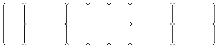
We go back to the assumption of symmetric tiles, but expand the corridor to dimensions . The recursion approach now seems to be problematic – it is possible to have patterns or arbitrary length that do not reduce to a shorter length, see figure 2.
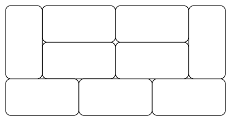
We thus instead look only at the right end of the tiling and argue that every tiling has to end with one of the three patterns depicted in the top row of figure 3.
Removing these end pieces either produces a tiling of length , or a tiling of length in which the top (or bottom) right corner is missing. We thus introduce a count for tilings of length with the top right corner missing, the count for the bottom right corner missing will by symmetry be the same. The three possible end cases thus give us the recursion
Since we also need no know the values of , we build a recursive formula for them as well. Consider a tiling with the top right corner missing. It’s right end must be a vertical tile or two horizontal tiles. In this second case there also will have to be a further horizontal tile in the top row; the ends thus look as in the bottom row of figure 3.
This gives us the recursion
We use the initial values , , , , , and thus get the following identities for the associate generating functions
and
We solve this second equation as
and substitute into the first equation, obtaining the functional equation
which we solve for
This is a function in , indicating that for odd (indeed, this must be, as in this case is odd and cannot be tiled with tiles of area ). We thus can consider instead the function
with . Partial fraction decomposition, geometric series, and final collection of coefficients gives us the formula
and the sequence of given by OEIS A001835
If we consider wider corridors the recursions become more complicated. It is therefore somewhat surprising that it is possible to give a general formula for the number of ways of tiling an rectangle with dominoes. According to [temperleyfisher], it is
but its derivation is beyond the scope of this course.
4 Catalan Numbers
The induction I used was pretty tedious, but I do not doubt that this result could be obtained much easier. Concerning the progression of the numbers 1, 2, 5, 14, 42, 132, etc. …
Die Induction aber, so ich gebraucht, war ziemlich mühsam, doch zweifle ich nicht, dass diese Sach nicht sollte weit leichter entwickelt werden können. Ueber die Progression der Zahlen 1, 2, 5, 14, 42, 132, etc. … Letter to Goldbach
September 4, 1751
Leonard Euler
Next, we look at an example of a recursion which is not linear; we also use what is essentially the product rule:
Definition 9.
The -th Catalan number444Named in honor of Eugène Charles Catalan (1814-1894) who first stated the standard formula. The naming after Catalan only stems from a 1968 book, see http://www.math.ucla.edu/~pak/papers/cathist4.png. Catalan himself attributed them to Segner, though Euler’s work is even earlier. OEIS A000108 is defined555Careful, some books use a shifted index, starting at only! as the number of different ways a sum of variables can be evaluated by inserting parentheses.
We have , : and , and :
To get a recursion, consider the position of the “outermost” addition: suppose it is after of the variables have been encountered. On its left side is a parenthesized expression in variables, on the ride side is an expression in variables. We thus get the recursion
in which we sum over the products of lower terms.
This is basically the pattern of the product rule, just shifted by one.
We thus get the functional equation
(which is easiest seen by writing out the expression for and collecting terms). The factor is due to the way we index and 1 is due to initial values.
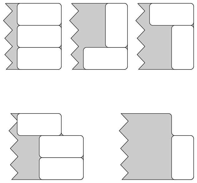
This is a quadratic equation in and yields the solution
The branch of the root was chosen so that the function has a limit, namely the value of , at . (The other branch yields a singularity, see Figure 4.)
The binomial series gives
We also observe that
Therefore
which shows that
Catalan numbers have many other combinatorial interpretations, and we shall encounter some in the exercises. Exercise 6.19 in [stanley2] (and its algebraic continuation 6.25, as well as an online supplement) contain hundreds of combinatorial interpretations.
5 Index-dependent coefficients and exponential generating functions
A recursion does not necessarily have constant coefficient, but might have a coefficient that is a polynomial in . In this situation we can use (formal) differentiation, which will convert a term into . The second derivative will give a term ; first and second derivative thus allow us to construct a coefficient and so on for higher order polynomials.
The functional equation for the generating function then becomes a differential equation, and we might hope that a solution for it can be found in the extensive literature on differential equations.
Alternatively, (using the special form of derivatives for a typical summand), such a situation often can be translated immediately to a generating function by using the power series
For an example of variable coefficients, we take the case of counting derangements OEIS A000166, that is permutations that leave no point fixed. We denote by the number of derangements on .
To build a recursion formula, suppose that is a derangement on . Then . We now distinguish two cases, depending on how is mapped by :
a) If , then swaps and and is a derangement of the remaining points, thus there are derangements that swap and . As there are choices for , there are derangements that swap with a smaller point.
b) Suppose there is such that . In this case we can “bend” into another permutation , by setting
We notice that is a derangement of the points .
Vice versa, if is a derangement on , and we choose a point , we can define on by
We again notice that is a derangement, and that different choices of and result in different ’s. Furthermore, the two constructions are mutually inverse, that is every derangement that is not in class a) is obtained by this construction.
There are possible derangements and choices for , so there are derangements in this second class.
We thus obtain a recursion
and hand-calculate666The reader might have an issue with the choice of , as it is unclear what a derangement on no points is. But we know that and , forcing this value for to make the recursion consistent. the initial values and .
From this recursion we could now construct a differential equation for the generating function of , but there is a problem: Because of the factor in the recursion, the values grow roughly like . The resulting series thus will have convergence radius , making it unlikely that a function satisfying this differential equation can be found in the literature.
We therefore introduce the exponential generating function which is defined simply by dividing the -th coefficient by a factor of , thus keeping coefficient growth bounded.
In our example, we get
and thus
We also have
From this, the recursion (written as ) gives:
and thus the separable differential equation
with .
Standard techniques from Calculus give the solution
of this differential equation. Looking up this function for Taylor coefficients (respectively determining the formula by induction) shows that
and thus (introducing a factor to make up for the denominator in the generating function) that
This is ,multiplied with a Taylor approximation of . Indeed, if we consider the difference to , the alternating series gives, for :
We have proven:
Lemma 5.1.
is the integer closest to .
That is asymptotically, if we put letters into envelopes, the probability is that no letter is in the correct envelope.
6 The product rule, revisited
Exponential generating functions have one more trick up their sleeve, arguably their most important contribution. For this, let us return to the product rule. It corresponds to the situation that the objects of a certain “weight”777The word “weight” indicates a size measurement, e.g. the number of vertices in a graph. can be described in terms of combining objects of lower weights (that sum up to the desired weight) in all possible ways.
This splitting-up however only considers the number of (sub)objects in each part, not which particular ones are in each part. In other words, we consider the constituent objects as indistinguishable.
Suppose now, however, that we are counting objects whose parts have identifying labels. In the example of the Catalan numbers this would be for example, if we cared not only about the parentheses placement, but also about the symbols we add, that is would be different from .
In such a situation, the recursion formula must, for each , account for which elements are chosen to be in the “left side”, with the rest being in the“right side”. Every combination is possible. That is, the recursion becomes:
We can write this as
which is the formula for multiplication of the exponential generating functions!
Let us look at this in a pathetic example, the number of functions from to (which we know already well as ).
Let count the number of constant functions on an -element set, that is . The associated exponential generating function thus is
(which, incidentally, shows why these are called “exponential” generating functions).
If we take an arbitrary function on , we can partition into (possibly empty) sets , such that is constant on and the are maximal with this property.
We get all possible functions by combining constant functions on the possible ’s for all possible partitions of . Note that the ordering of the partitions is significant – they indicate the actual values.
We are thus exactly in the situation described, and get as exponential generating function (start with , then use induction for larger ) the -fold product of the exponential generating functions for the number of constant functions:
The coefficient for in the power series for is , and hence the counting function is , as expected.
1 Bell Numbers
The integral -squared d,
From one to the cube root of three,
Times the cosine,
Of three pi over nine
Equals log of the cube root of e.
Anon.
We try this approach next to obtain an exponential generating function for the Bell numbers (though not a closed form expression for its coefficients):
Recall that the Bell numbers give the total number of partitions of and satisfy (Lemma 0.1) the recursion:
In light of the product rule, we insert a factor 1 and write this (after reindexing) as
and thus
If we denote the exponential generating function of the by , the right hand side thus will give the product of the generating function of the constant sequence (which we just saw is ) with . This reflects the split that gave us the recursion – into a set of size containing the number (the total number of such sets being once the numbers are chosen), and a partition of the remaining numbers.
The left hand side is the exponential generating function of which is just the derivative of , thus we have that
This is a separable differential equation, it’s solution is
for some constant . As we solve for and hence get the exponential generating function
There is no nice way to express the power series coefficients of this function in closed form, a Taylor approximation is (with denominators being deliberately kept in the form of to allow reading off the Bell numbers):
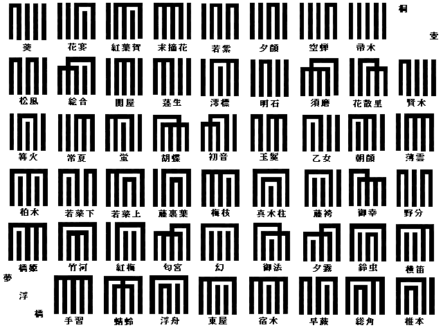
One, somewhat surprising, application of Bell numbers is to consider rhyme schemes. Given a sequence of lines, the lines which rhyme form the cells of a partition of . For example, the partition is the scheme AABBA used by Limericks, while Poe’s The Raven uses AABCCCBBB or
We can read off the Taylor expansion that . The classic 11th century Japanese novel Genji monogatari (The Tale of Genji) has 54 chapters of which first and last are considered “extra”. The remaining 52 chapters are introduced each with a 5 line poem in one of the 52 possible rhyme schemes and a symbol illustrating the scheme. These symbols, see figure 5, the Genji-mon, have been used extensively in Art. See https://www.viewingjapaneseprints.net/texts/topics_faq/genjimon.html
2 Stirling numbers
We apply the same idea to the Stirling numbers of the second kind, denoting the number of partitions of into (non-empty) parts. According to 8, part 3) there are order-significant partitions of into parts.
We denote the associated exponential generating function (for order-significant partitions) by
We also know that there is – apart from the empty set – exactly one partition into one cell. That is
If we have a partition into -parts, we can fix the first cell and then partition the rest further. Thus, for we have that
which immediately gives that
We deduce that the Stirling numbers of the second kind have the exponential generating function
Using the fact that , we thus get the exponential generating function for the Bell numbers as
in agreement with the above result.
We also can use the exponential generating function for the Stirling numbers to deduce a coefficient formula for them:
Lemma 6.1.
Proof 6.2.
We first note that – as – the -sum could start at or alternatively without changing the result.
Then multiplying through with , we know by the binomial formula that
and we read off the coefficients.
3 Involutions
Finally, let us use this in a new situation:
Definition 10.
A permutation on is called888Group theorists often exclude the identity, but it is convenient to allow it here. an involution OEIS A000085 if , i.e. for all .
We want to determine the number of involutions on points.
Consider the number of cycles (including -cycles, that is fixed points). Let be the number of involutions with exactly cycles. Clearly , , , , hence the exponential generating function for a single cycle is .
When considering an arbitrary involution, we can split off a cycle, seemingly leading to a formula
But (similar as when we considered a generating function for for the Stirling numbers), such a product of exponential generating functions will consider the arrangement of cycles, i.e. consider different from . We correct this by dividing by and thus get
and thus for the exponential generating function of the number of involutions a sum over all possible :
We easily write down a power series for the two factors
and multiply out, yielding
and thus (again introducing a factor of for making up for the exponential generating function)
Chapter 3 Inclusion, Incidence, and Inversion
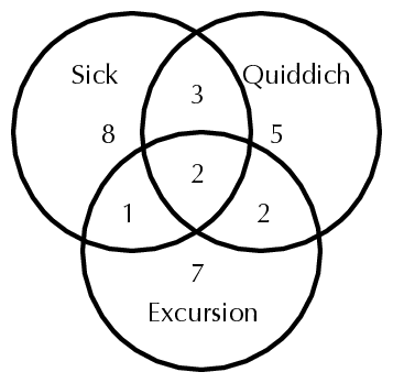
It is calculus exam week and, as every time, a number of students were reported to require alternate accommodations:
-
•
students are sick.
-
•
students are scheduled to play for the university Quiddich team at the county tournament.
-
•
students are planning to go on the restaurant excursion for the food appreciation class.
-
•
students on the Quiddich team are sick (having been hit by balls).
-
•
students are scheduled for the excursion and the tournament.
-
•
students of the food appreciation class are sick (with food poisoning), and
-
•
of these students also planned to go to the tournament, i.e. have all three excuses.
The course coordinator wonders how many alternate exams need to be provided.
Using a Venn diagram and some trial-and-error, it is not hard to come up with the diagram in figure 1, showing that there are alternate exams to offer.
1 The Principle of Inclusion and Exclusion
By the method of exclusion,
I had arrived at this result,
for no other
hypothesis would meet the facts.
A Study in Scarlet
Arthur Conan Doyle
The Principle of Inclusion and Exclusion (PIE) formalizes this process for an arbitrary number of sets:
Let be a set and a family of subsets. For any subset we define
using that . Then
Lemma 1.1.
The number of elements that lie in none of the subsets is given by
Proof 1.2.
Take and consider the contribution of this element to the given sum. If for any , it only is counted for , that is contributes .
Otherwise let and let . We have that if and only if . Thus contributes
As a first application we determine the number of derangements on points in an different way:
Let be the set of all permutations of degree , and let be the set of all permutations with . Then is exactly the set of derangements, there are possibilities to intersect of the ’s, and the formula gives us:
For a second example, we calculate the number of surjective mappings from an -set to a -set (which we know already from 8 to be ):
Let be the set of all mappings from to , then . Let be the set of those mappings , such that is not in the image of , so . More generally, if we have that . The surjective mappings are exactly those in outside any of the , thus the formula gives us the count
using again that there are possible sets of cardinality .
The factor in a formula often is a good indication that inclusion/exclusion is to be used.
Lemma 1.3.
Proof 1.4.
To use PIE, the sets need to involve choosing from an , set, and after choosing of these we must choose from a set of size .
Consider a bucket filled with blue balls, labeled with , and red balls. How many selections of balls only involve red balls? Clearly the answer is the right hand side of the formula.
Let be the set of all -subsets of balls and those subsets that contain blue ball number , then PIE gives the left side of the formula.
We finish this section with an application from number theory. The Euler function counts the number of integers with .
Suppose that , and the integers in that are multiples of . Thus and for we have that consists of multiples of and thus . Then counts the number of elements in that do not lie in any of the and (inclusion/exclusion)
with the second identity obtained by multiplying out the product on the right hand side.
We also note – exercise LABEL:phisum – that . On its own this looks as if it is entirely separate from the inclusion/exclusion concept we just considered. But by generalize the concept of a hierarchy, given hitherto through inclusion of subsets, to more general situations, we shall see that this is a structural consequence of the previous formula.
2 Partially Ordered Sets and Lattices
The doors are open; and the surfeited grooms
Do mock their charge with snores:
I have drugg’d their possets,
That death and nature do contend about them
Macbeth, Act II, Scene II
William Shakespeare
A poset or partially ordered set is a set with a relation on the elements of which we will typically write as instead of , such that for all :
- (reflexive)
-
.
- (antisymmetric)
-
and imply that .
- (transitive)
-
and imply that .
The elements of a poset thus are the elements of , not those of the underlying relation and is cardinality is that of .
For example, could be the set of subsets of a particular set, and with be the “subset or equal” relation.
A convenient way do describe a poset for a finite set is by its Hasse-diagram. Say that covers if , and there is no with . The Hasse diagram of the poset is a graph in the plane which connects two vertices and only if covers , and in this case the edge from to goes upwards.
Because of transitivity, we have that if and only if one can go up along edges from to reach .
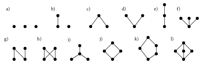
Figure 2 gives a number of examples of posets, given by their Hasse diagrams, including all posets on 3 elements.
An isomorphism of posets is a bijection that preserves the relation.
An element in a poset is called maximal if there is no larger (wrt. ) element, minimal is defined in the same way. Posets might have multiple maximal and minimal elements.
For another cute example 111Taken from lecture notes [axue] consider in Figure 3, left, the arrangement of fruits according to convenience and taste, as given by222pardon the title of the cartoon https://xkcd.com/388/.
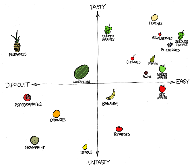
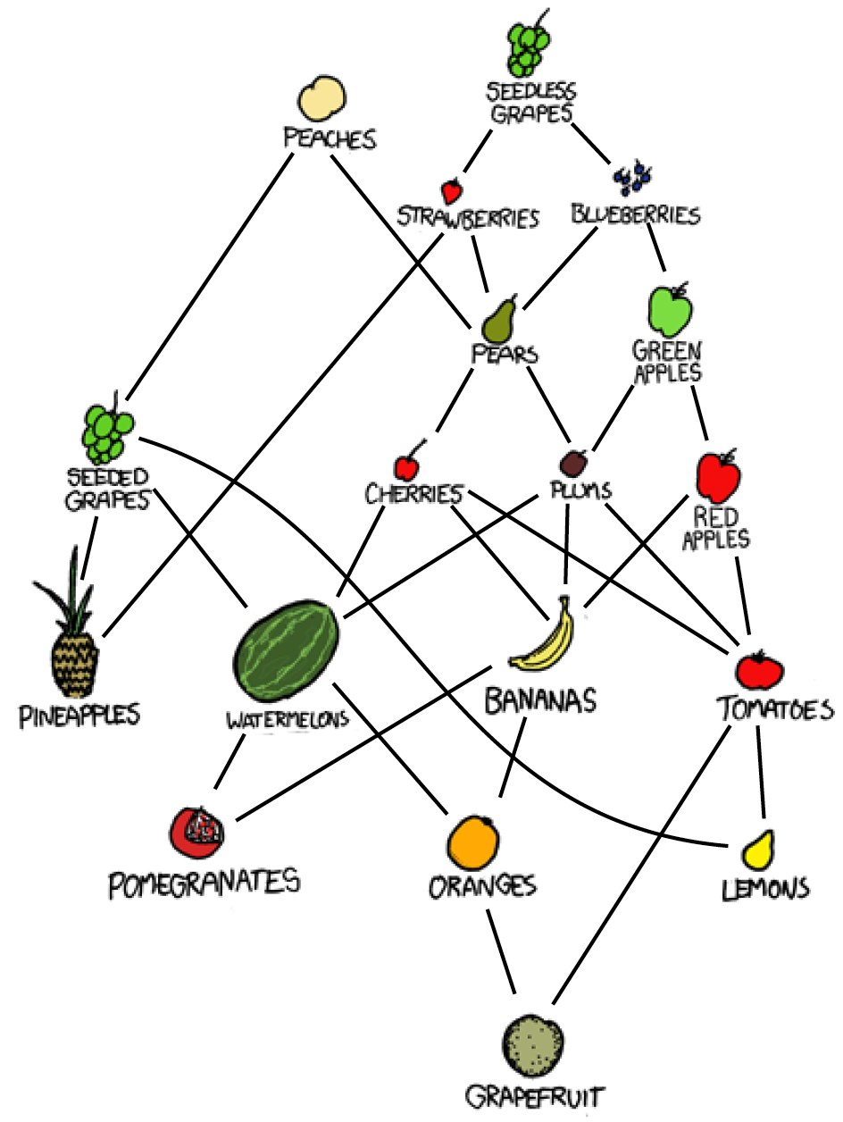
R. Munroe, F*** Grapefruit, https://xkcd.com/388/, and [axue], p.108
We can read of a partial order from this by declaring a fruit as “better” than another, if it both more tasty and easier to consume. The resulting Hasse diagram is on the right side of Figure 3. It is easily seen that not every pair of fruits is comparable this way, and that there is no universal “best” or “worst” fruit.
1 Linear extension
My scheme of Order gave me the most trouble
Autobiography
Benjamin Franklin
A partial order is called a total order, if for every pair of elements we have that or .
While this is not part of our definition, we can always embed a partial order into a total order.
Proposition 11.
Let be a partial order on . Then there exists a total order (called a linear extension) such that .
To avoid set acrobatics we shall prove this only in the case of a finite set . Note that in Computer science the process of finding such an embedding is called a topological sorting.
Proof 2.1.
We proceed by induction over the number of pairs that are incomparable. In the base case we already have a total order.
Otherwise, let such an incomparable pair. We set (arbitrarily) that . Now let
We claim that is a partial order. As it has fewer incomparable pairs, this shows by induction that there exists a total order , proving the theorem.
Since is reflexive, is. For antisymmetry, suppose by contradiction that for some we have that . Since is a partial order, not both could have been in .
Thus assume (WLOG) that
This implies that and . If , this implies by transitivity that , contradicting the choice of . If , then also and thus by definition . Transitivity implies again in contradiction to the choice of .
For transitivity, the definition of implies that we cannot have transitivity for pairs in . Thus first suppose that and . Then , as otherwise . But then , implying that . The other remaining case is analog.
This theorem implies that we can always label the elements of a countable poset with positive integers, such that the poset ordering implies the integer ordering. Such an embedding is in general not unique, see Theorem 21.
The case of a totally ordered subset gets a special name:
Definition 12.
A chain in a poset is a subset of such that any two elements of it are comparable. (That is, restricted to the chain the order is total.)
2 Lattices
Definition 13.
Let be a poset and .
-
•
A greatest lower bound of and is an element which is maximal in the set of elements with this property.
-
•
A least upper bound of and is an element which is minimal in the set of elements with this property.
is a lattice if any pair have a unique greatest lower bound, called the meet and denoted by ; as well as unique least upper bound, called the join and denoted by .
Amongst the Hasse diagrams in figure 2, e,j,k,l) are lattices, while the others are not. Lattices always have unique maximal and minimal elements, sometimes denoted by (minimal) and (maximal).
Other examples of lattices are:
-
1.
Given a set , let the power set of with defined by inclusion. Meet is the intersection, join the union of subsets.
-
2.
Given an integer , let be the set of divisors of with given by “divides”. Meet and join are , respectively lcm.
-
3.
For an algebraic structure , let be the set of all substructures (e.g. group and subgroups) of and given by inclusion. Meet is the intersection, join the substructure spanned by the two constituents.
-
4.
For particular algebraic structures there might be classes of substructures that are closed under meet and join, e.g. normal subgroups. These then form a (sub)lattice.
Using meet and join as binary operations, we can axiomatize the structure of a lattice:
Proposition 14.
Let be a set with two binary operations and and two distinguished elements . Then is a lattice if and only if the following axioms are satisfies for all :
- Associativity:
-
and ;
- Commutativity:
-
and ;
- Idempotence:
-
and ;
- Inclusion:
-
;
- Maximality:
-
and .
Proof 2.2.
The verification that these axioms hold for a lattice is left as exercise to the reader.
Vice versa, assume that these axioms hold. We need to produce a poset structure and thus define that iff . Using commutativity and inclusion this implies the dual property that .
To show that is a partial order, idempotence shows reflexivity. If and then and thus antisymmetry. Finally suppose that and , that is and . Then
and thus . Associativity gives us that if also then
and thus , thus is the unique greatest lower bound. The least upper bound is proven in the same way and the last axiom shows that is the unique minimal and the unique maximal element.
Definition 15.
An element of a lattice is join-irreducible (JI) if and if implies that or .
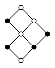
For example, figure 4 shows a lattice in which the black vertices are JI, the others not.
If we take the lattice of subsets of a set, the join-irreducibles are the 1-element sets. If we take divisors of , the join-irreducibles are prime powers.
When representing elements of a finite lattices, it is possible to do so by storing the JI elements once and representing every element based on the JI elements that are below. This is used for example in one of the algorithms for calculating the subgroups of a group.
3 Product of posets
The cartesian product provides a way to construct new posets (or lattices) from old ones: Suppose that are posets with orderings , , we define a partial order on by setting
Proposition 16.
This is a partial ordering, so is a poset. If furthermore both and are lattices, then so is .
The proof of this is exercise LABEL:posetproduct.
This allows us to describe two familiar lattices as constructed from smaller pieces (with a proof also delegated to the exercises):
Proposition 17.
a) Let and the power-set lattice (that is the subsets
of , sorted by inclusion). Then is (isomorphic to) the
direct product of copies of the two element lattice .
b) For an integer written as a product of
powers of distinct primes, let be the lattice of divisors of
. Then .
3 Distributive Lattices
A lattice is distributive, if for any one (and thus also the other) of the two following laws hold:
These laws clearly hold for the lattice of subsets of a set or the lattice of divisors of an integer .
Lattices of substructures of algebraic structures are typically not distributive, the easiest example (diagram l) in figure 2) is the lattice of subgroups of which also is the lattice of subspaces of .
If is a poset, a subset is an order ideal, if for any and we have that implies .
Lemma 3.1.
The set of order ideals is closed under union and intersection.
Proof 3.2.
Let be order ideals and and . Then or . In the first case we have that , in the second case that , and thus always . The same argument also works for intersections.
This implies:
Lemma 3.3.
The set of order ideals of , denoted by is a lattice under intersection and union.
As a sublattice of the lattice of subsets, is clearly distributive.
For example, if is the poset on 4 elements with a Hasse diagram given by the letter (figure 2, g) then figure 4 describes the lattice .
In fact, any finite distributive lattice can be obtained this way
Theorem 18 (Fundamental Theorem for Finite Distributive Lattices, Birkhoff).
Let be a finite distributive lattice. Then there is a unique (up to isomorphism) finite poset , such that .
To prove this theorem we use the following definition:
Definition 19.
For any element of the poset , let be the principal order ideal generated by .
Lemma 3.4.
An order ideal of a finite poset is join irreducible in if and only it is principal.
Proof 3.5.
First consider a principal order ideal and suppose that with and being order ideals. Then or , which by the order ideal property implies that or .
Vice versa, suppose that is a join irreducible order ideal and assume that is not principal. Then for any , is a proper subset of . But clearly .
Corollary 20.
Given a finite poset , the set of join-irreducibles of , considered as a subposet of , is isomorphic to .
Proof 3.6.
Consider the map that maps to . It maps bijective to the set of join-irreducibles, and clearly preserves inclusion.
We now can prove theorem 18
Proof 3.7.
Given a distributive lattice , let be the set of join-irreducible elements of and be the subposet of formed by them. By corollary 20, this is the only option for up to isomorphism, which will show uniqueness.
Let be defined by , that is it assigns to every element of the JI elements below it. (Note that indeed is an order ideal.). We want to show that is an isomorphism of lattices.
Step1: Clearly we have that for any (using the join over the empty set equal to ). Thus is injective.
Step 2: To show that is surjective, let be an order ideal of , and let . We aim to show that : Clearly every also has , so . Next take a join irreducible , that is . Then and thus
by the distributive law. Because is JI, we must have that for some , implying that . But as is an order ideal this implies that . Thus and thus equality, showing that is surjective.
Step 3: We finally need to show that maps the lattice operations: Let . Then if and only if and . Thus .
For the join, take . Then , implying , or (same argument) ; therefore . Vice versa, suppose that , so and thus
Because is JI that implies , respectively .
In the first case this gives and thus ; the second case similarly gives .
We close with a further use of the order ideal lattice:
Theorem 21.
Let be a poset of size . The number of different linear orderings of is equal to the number of different chains of (maximal) length in .
Proof 3.8.
Exercise.
4 Chains, Antichains, and Extremal Set Theory
Man is born free;
and everywhere he is in chains
The Social Contract
Jean-Jacques Rousseau
We start with a definition dual to that of a chain:
Definition 22.
An antichain in a poset is a subset, such that any two (different) elements are incomparable.
We shall consider partitions of (the elements of) a poset into a collection of chains (or of antichains).
Clearly a chain and antichain can intersect in at most one element. This gives the following duality:
Lemma 4.1.
Let be a poset.
a) If has a chain of size , then it cannot be partitioned in fewer
than antichains.
b) If has an antichain of size , then it cannot be partitioned in
fewer than chains.
A stronger version of this goes usually under the name of Dilworth’s theorem333proven earlier by Gallai and Milgram.
Theorem 23 (Dilworth, 1950).
The minimum number of chains in a partition of a finite poset is equal to the maximum number of elements in an antichain.
Proof 4.2.
The previous lemma shows that , so we only need to show that we can partition into chains. We use induction on , in the base case nothing needs to be shown.
Consider a chain in of maximal size. If every antichain in contains at most elements, we apply induction and partition into chains and are done.
Thus assume now that was an antichain in . Let
Then , as there otherwise would be an element we could add to the antichain and increase its size.
As is of maximal size, the largest element of cannot be in , and thus we can apply induction to . As there is an antichain of cardinality in , we partition into disjoint chains.
Similarly we partition into disjoint chains. But each is maximal element of exactly one chain in and minimal element of exactly one chain of . We can combine these chains at the ’s and thus partition into chains.
Corollary 24.
If is a poset with elements, it has a chain of size or an antichain of size .
Proof 4.3.
Suppose not, then every antichain has at most elements and by Dilworth’s theorem we can partition into chains of size each, so .
Corollary 25 (Erdős-Szekeres, 1935).
Every sequence of distinct integers contains an increasing subsequence of length at least , or a decreasing subsequence of at length least .
Proof 4.4.
Suppose the sequence is with . We construct a poset on elements by defining if and only if and . (Verify that it is a partial order!)
The theorems of this section in fact belong into a bigger context that has its own chapter, chapter 4, devoted to.
A similar argument applies in the following two famous theorems, that are part of foundational material of extremal set theory.
Theorem 26 (Sperner, 1928).
Let and , such that if . Then .
Proof 4.5.
Consider the poset of subsets of and let . Then is an antichain.
A maximal chain in this poset will consist of sets that iteratively add one new point, so there are maximal chains, and maximal chains that involve a particular -subset of .
We now count the pairs such that and is a maximal chain with . As a chain can contain at most one element of an antichain this is at most .
On the other hand, denoting by the number of sets with , we know there are
such pairs. As is maximal for we get
We note that equality is achieved if is the set of all -subsets of .
Theorem 27 (Erdős-Ko-Rado, 1961).
Let a collection of distinct -subsets of , where , such that any two subsets have nonempty intersection. Then .
Proof 4.6.
Consider “cyclic -sequences” with , taken “modulo ” (that is each number should be ).
Note that , since if some equals , then any only other must intersect , so we only need to consider (again considering indices modulo ) for . But will not intersect , allowing at most for a set of subsequent ’s to be in .
As this holds for an arbitrary , the result remains true after applying any arbitrary permutation to the numbers in . Thus
We now calculate the sum by fixing , and observe that there are permutations such that . Thus , proving the theorem.
5 Incidence Algebras and Möbius Functions
A common tool in mathematics is to consider instead of a set the set of functions defined on . To use this paradigm for (finite) posets, define an interval on a poset for a given pair as the set , and denote by the set of all intervals. (It might be convenient to set if .
For a field , we shall consider the set of functions on the intervals:
(with ) and call it the incidence algebra of . If we denote intervals by their end points , we shall write for if .
This set of functions is obviously a -vector space under pointwise operations. We also define a multiplication on by defining, for a function by
In exercise LABEL:incidencealgebra we will show that with this definition becomes an associative -algebra444An algebra is a structure that is both a vector space and a ring, such that vector space and ring operations interact as one would expect. The prototype is the set of matrices over a field. with a one, given by
We could consider as the set of formal -linear combinations of intervals and a product defined by
and extended bilinearily.
If is finite, we can, by theorem 11, arrange the elements of as where implies that . Then is, by exercise LABEL:incalgmatalg isomorphic to the algebra of upper triangular matrices where if .
Lemma 5.1.
Let . Then has a (two-sided) inverse if and only if for all .
Proof 5.2.
The property is equivalent to:
(implying the necessity of ) and
If the second formula will define the values uniquely, depending only on the interval . Reverting the roles of and shows the existence of a left inverse and standard algebra shows that both have to be equal.
The zeta function of is the characteristic function of the underlying relation, that is if and only if (and ).
This implies that
is the size of the interval.
By Lemma 5.1, is invertible. The inverse is called the Möbius function of the lattice . The identities
| (1) | |||||
| (2) |
follow from and allow for a recursive computation of values of and imply that is integer-valued.
For illustration, we shall compute the Möbius function for a number of common posets.
Lemma 5.3.
Let be the total order on the numbers . Then for any we have:
Proof 5.4.
The case of is trivial. If , the sum in 2 has only one summand, and the result follows. Thus assume that but . Then
and the result follows by induction on .
Lemma 5.5.
If , are posets, the Möbius function on satisfies
Proof 5.6.
It is sufficient to verify that the right hand side of the equation satisfies 2.
Corollary 28.
a) For , we have that
if , and 0 otherwise.
b) If are divisors of , then in we have that
if is the product of different primes, and 0
otherwise.
Part b) explains the name: is the value of the classical number theoretic Möbius function.
Part a) connects us back to section 1: The Möbius function gives the coefficients for inclusion/exclusion over an arbitrary poset. We will investigate and clarify this further in the rest of this section.
1 Möbius inversion
The property of being inverse of the incidence function can be used to invert summation formulas with the aid of the Möbius function:
Theorem 29 (Möbius inversion formula).
Let be a finite poset, and , where is a field. Then
is equivalent to
Proof 5.7.
Let be the -vector space of functions . The incidence algebra acts linearly on this vector space by
The two equations thus become
and their equivalence follows from the fact that is the inverse of .
The classical Möbius inversion formula from Number Theory follows as a special case of this.
If we consider the linear poset with total ordering, Lemma 5.3 gives us that (we assume ) the (unsurprisingly) result that
is equivalent to
the finite difference analog of the fundamental theorem of Calculus!
Going back to the start of the chapter, consider subsets of a set . We take the the poset and define, for
Then by Inclusion/Exclusion over the complements , while
is the ordinary inclusion/exclusion formula.
Chapter 4 Connections
Mathematicians are like Frenchmen.
When you talk to them, they translate
it into their own language,
and then it is something quite different.
Die Mathematiker sind eine Art Franzosen;
redet man zu ihnen, so übersetzen sie es
in ihre Sprache, und dann ist es
alsobald ganz etwas anders. Maximen und Reflexionen:
Über Natur und Naturwissenschaft
Johann Wolfgang von Goethe
With so many joints and connections, leaks were plentiful. As the magazine
The Builder remarked, in 1856: “The fate of a theater is to be
burned. It seems simply a question of time.”
Connections
James Burke
In this chapter we will look at connections – both in an applied sense of modeling situations of connected objects, in the abstract sense of connecting mathematical theorems that initially seem to be unrelated, and in connecting concepts that might seem to be hopelessly abstract to practical applications. One of the joys of mathematics is to discover such connections and see the unity of the discipline.
This practical relevance of the results places much of this chapter also in close contact to the realm of (discrete) optimization.
We shall investigate a gaggle of theorems (which each in their area are fundamental), but which turn out to be equivalent in the sense that we can deduce each theorem as a consequence from any other. Furthermore this kind of derivation is often easier than to derive the theorem from scratch. The description owes much to [reichmeider]
Many theorems in this chapter are formulated in the language of graphs: We typically denote a graph by with vertices and edges being 2-element sets of vertices. A digraph is a graph with directed edges (that is we consider edges as elements of instead of -element subsets of ). In a digraph, we would allow distinct edges and . Weighted edges means we have a weight function .
Our start will be Dilworth’s Theorem 23 that we have proven already:
The minimum number of chains in a partition of a finite poset is equal to the maximum number of elements in an antichain.
1 Halls’ Marriage Theorem
He was, methinks, an understanding fellow who said, ’twas a happy marriage betwixt a blind wife and a deaf husband.
Celuy là s’y entendoit, ce me semble, qui dict qu’un bon mariage se dressoit d’une femme aveugle avec un mary sourd. Essais, Livre III
Michel de Montaigne
Consider a family of subsets . A system of distinct representatives (SDR) for these sets is an -tuple of distinct elements such that .
SDRs do not have to exist, for example consider .
We define, for a subset of indices, a set
We immediately see a reason for the above example failing: For an SDR to exist, by necessity for any such subset , since there are otherwise not sufficiently many elements available to pick distinct representatives. The following Theorem111Proven by the British Mathematician Philip Hall and extended by the unrelated American Mathematician Marshall Hall for the infinite case. Thus the apostrophe placement in the section title. shows this condition is not only necessary, but also sufficient.
Theorem 30 (Halls’ Marriage Theorem).
The family of finite sets has a system of distinct representatives if and only if
| (1) |
The name “Marriage Theorem” comes from the following interpretation: Suppose we have a set of men and women. We let be the set of men that women would consider for a potential marriage222The theorem goes back to times of more restrictive social mores. The concerned reader might want to consider applicants for jobs and being the set of candidates that satisfy the conditions for job .. Then every women can marry a suitable man if and only if every group of women together considers at least men as suitable.
Proof 1.1 (DilworthHall).
As the necessity of the condition is trivial, we show sufficiency:
Given sets satisfying condition (1), Let be symbols representing the sets. We create a poset in the following way: The elements of is the disjoint union . The only relations are that iff .
Clearly is an antichain in . Suppose is another arbitrary antichain and let . The antichain criterion imposes that , so
because of (1). That means is a maximal antichain, and by Dilworth’s theorem, can be partitioned into chains. As a chain cannot contain more than one point from or more than one point from , the pigeonhole principle implies that each chain contains exactly one point from and at most one point from . Suppose that is the element that is together with in a chain. Then , and thus , so is a SDR.
As an example of the use of this theorem we consider the following theorem due to G. Birkhoff. A matrix with nonnegative entries is called doubly statistic333There also is the term doubly stochastic, which denotes real matrices with row/column sum 1. I.e. every double statistic matrix can be scaled to a double stochastic matrix if every row and every column of has the same row/column sum.
Corollary 31.
A doubly statistic matrix with row/column sum can be written as the sum of permutation matrices.
Proof 1.2.
We define sets , corresponding to the row indices by . For any -tuple of indices, the sum of the corresponding rows of is . As every column of has column sum , this means that these rows must have nonzero entries in at least columns, that is . Thus 1 is satisfied and there is a SDR. We set if is the chosen representative for (and otherwise). Then is a permutation matrix and is doubly statistic with sum . The statement follows by induction on .
2 Kőnig’s Theorems – Matchings
Eventually everything connects - people, ideas, objects…the quality of the connections is the key to quality per se. Charles Eames
Let be an matrix with entries. A line of is a row or column. A set of lines covers , if every nonzero entry of lies on at least one of the lines. Nonzero entries are called independent if no two lie on a common line. The term rank of is the maximum number of independent entries of .
The following theorem is reminiscent of the properties of a basis in linear algebra:
Theorem 32 (Kőnig-Egerváry).
The minimum number of lines covering equals the term rank of .
Let
Then can be covered with lines, and has an independent set of cardinality .
Proof 2.1 (HallKőnig-Egerváry).
Given , let be the term rank of and the minimum number of lines covering . We have to show that .
We first show that : A cover of lines can cover at most independent ’s (no line covers more than one) but we can cover all ones with lines, so .
To see that , without loss of generality permute the rows and columns of such that a minimal cover involves the first rows and the last columns of the matrix. We aim to find an independent set that has entries in the first rows and in columns , and entries in the last columns in rows :
For a row index let . Then the union of any of these ’s contains at least column indices – otherwise we could replace these rows with columns in a minimal cover. By Hall’s theorem we thus have an SDR . By definition implies that . Let . Since the are distinct, this is an independent set.
A dual argument for the last columns gives an independent set of positions in the last columns and rows . Since no position in shares row or column index with any position in , also is an independent set, of cardinality .
We reformulate this theorem in the language of graphs. A graph is called bipartite, if its vertex set can be written as a disjoint union , so that no vertex in has a neighbor in (but only neighbors in ). A vertex cover in a graph is a set of vertices that every edge is incident to at least one vertex in the cover. A matching in a graph is a set of edges such that no two edges are incident to the same vertex. A matching is called maximal, if no matching with a larger number of edges exists.
We assume that the graphs we consider here have no isolated vertices.
Theorem 33 (Kőnig).
In a bipartite graph without isolated vertices, the number of edges in a maximum matching equals the number of vertices in a minimum vertex cover.
Figure 1 shows a bipartite graph with a maximum matching (bold).
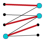
Proof 2.2 (Kőnig-EgerváryKőnig).
Let be the two parts of the bipartition of vertices. Suppose , . We describe the adjacency in an matrix with entries, iff is adjacent to . (Note that the examples for this and the previous theorem are illustrating such a situation.)
A matching in the graph corresponds to an independent set — edges sharing no common vertices. A vertex cover — vertices such that every edge is incident — correspond to a line cover of the matrix. The result follows immediately from the Kőnig-Egerváry theorem.
Matchings in bipartite graphs can be interpreted as creating assignments between tasks and operators, between customers and producers, between men and women, etc., and thus clearly have practical implications (Compare the Marriage Theorem interpretation of Hall’s theorem!)
Due to this practical relevance, there is obvious interest in an algorithm for finding maximum matchings in a bipartite graph, the Assignment problem. The first algorithm published uses Kőnig’s theorem as a criterion whether an existing matching can be improved. Due to the origin of the theorem authors, it has been named the Hungarian Method. (It turns out that this method had been discovered before independently by Jacobi [jacobiassign].)
Let be a (not necessarily maximal) matching in a graph . We call an edge matched if it is in , and free otherwise. Similarly, vertices incident to matched edges are called matched, vertices not incident to any matched edge are free.
An augmenting path for is a path whose end points are free and whose edges are alternatingly matched and free. This means all vertices but the end points are matched. Such a path allows us to replace with a larger matching, in that we can replace the matched edges of the augmenting path in with the free edges in the path, of which there is one more.
If the cardinality of is that of a vertex cover , of course no augmenting paths can exist: Every edge of will be incident with exactly one vertex in , leaving one of the two free edges at the end of the path without cover.
But if the cardinality is smaller there must be an augmenting path:
Corollary 34.
If for a vertex cover , there either is a vertex cover of smaller size, or there is an augmenting path for .
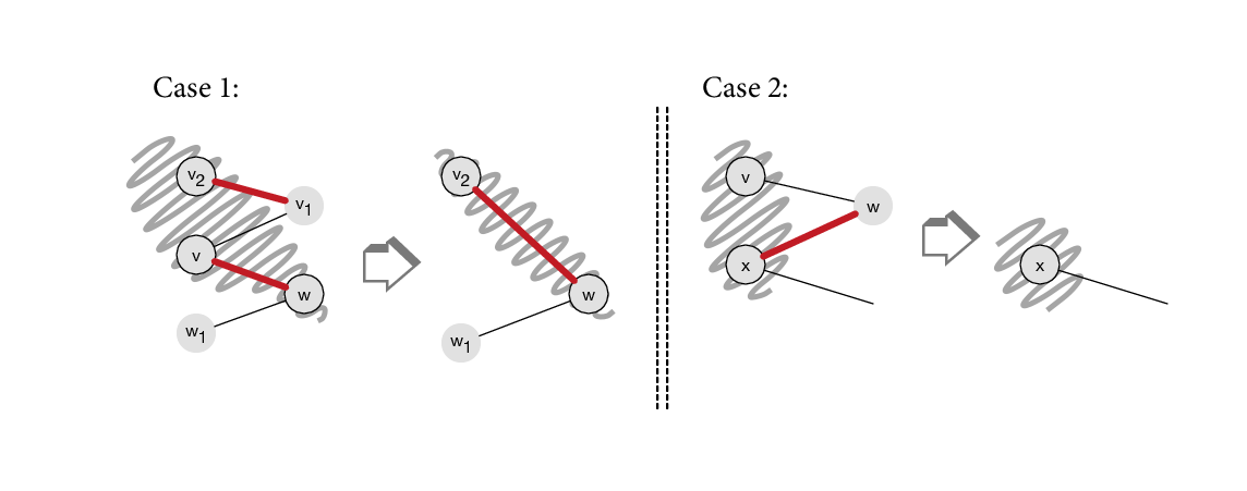
Proof 2.3.
We prove the statement by induction over the number of vertices , the base case being trivial.
Case 1: Assume that two vertices are connected by an edge in . Then both and must be incident to other edges, as we otherwise could drop one of them from and obtain a strictly smaller cover.
Furthermore one such edge must be to a vertex (as we otherwise could drop from the vertex cover). Clearly is free. We similarly find a free edge to a vertex . If both and are free, then is an augmenting path. Otherwise at least one vertex, WLOG , is matched thus incident to an edge . As we assumed that this implies that . As the graph is bipartite we also know that . Now consider the smaller graph obtained from by deleting and (and the adjacent edges) and adding an edge if it did not yet exist. Then is a matching in and a vertex cover in (see Figure 2, left). By induction, we can either obtain a strictly smaller vertex cover for (in which case or is a strictly smaller cover for ), or an augmenting path for . If this path uses the new matching edge , we replace this edge by the edge sequence and obtain an augmenting path in . This completes case 1.
In Case 2, we now may assume that no two vertices of the cover are connected by an edge in the matching, as there must be an unmatched vertex .
If is adjacent to any other unmatched vertex this is an augmented path of length .
Otherwise is adjacent to a matched vertex (if all neighbors are in , we could remove from ). By a matched edge, is adjacent to another vertex , and to cover that edge we must have . We furthermore may assume that was chosen so that is also incident to an edge not in the matching, as we otherwise could replace all ’s with the respective ’s in the cover and remove from , reducing the cover size.
Now consider the graph , obtained by removing the vertices and and their incident edges and set and (Figure 2, right).
Then is a vertex cover of (all edges that covered are gone). Also is a matching with . By induction, either has a smaller cover (in which case is a smaller cover for ), or there is an augmenting path. If this path imvolves , we extend it by and thus obtain an augmenting path for .
To find a maximal matching, one can thus simply start with some arbitrary matching (pick edges as long as no two share a vertex) and vertex cover and then use corollary 34 to refine them iteratively.
It is not hard to generalize this approach to (complete) bipartite graphs with weighted edges to obtain a (perfect: all vertices are matched) matching of maximal weight (profit):
Given an arbitrary matching with weighted edges, replace an edge with (assume: integral) weight by a set of edges with newly introduced vertices that are not connected in any other way. Selecting the edge in the original graph thus now allows selection of edges. Thus the maximum weight of a matching in the original graph corresponds to the cardinality of a maximum matching in the new graph.
1 Stable Matchings
…to Alvin E. Roth and Lloyd S. Shapley “for the theory of stable allocations and the practice of market design”. Citation for the Sveriges Riksbank Prize in Economic Sciences in Memory of Alfred Nobel 2012
Also of practical interest is the concept of a stable matching (or stable marriage). Imagine a matching in a bipartite graph represents an assignment of students to college places. Every student has a personal preference ranking of colleges, every college (place – assume for simplicity that every college just has one student) has a personal ranking of students. A matching is instable (otherwise: stable), if there is a student and a college such that ranks higher than their current college, and ranks higher than their current student.
A priori it is unclear that stable matchings exist, the following algorithm not only proves that but also gives a way of producing one:
[Deferred Acceptance, Gale, Shapley] Every student has a temporarily assigned college, colleges may have a temporarily assigned student. Once a college has been assigned a student, it will replace it only by one it ranks higher. A student may be moved down from higher ranked to lower ranked colleges.
For bookkeeping, students carry a rejected label that will change status as the algorithm goes on, and also and carry for each college an indicator whether they have been rejected by this college.
-
1.
[Initialize] Label every student as rejected
-
2.
[Complete] If no student is rejected, terminate.
-
3.
[Student Choice] Every student marked as rejected applies to the college she ranks highest amongst those who have not yet rejected her.
-
4.
[College Choice] Every college tentatively picks from the students who chose it the one it ranks highest (and removes that students rejection status). It rejects all other students who have selected it,even if they had been picked tentatively before.
-
5.
Go back to step 2.
Proof 2.4.
The only way the process terminates is if no student is rejected, that is they were tentatively accepted by a college and this college has no student applying it would rank higher. All colleges which the student ranks higher have rejected her because they were able to accept a student they rank higher, so the matching is stable.
In every round, students select from colleges and are either tentatively accepted, or are left with colleges of lower preference. As there is a finite set of students and preferences, this process must terminate.
This algorithm is used for example in the US to match graduating medical doctors to hospital training positions, www.nrmp.org. It also was instrumental for the award of the 2012 Nobel prize in Economics to Shapley and Roth.
3 Menger’s theorem
Live in fragments no longer. Only connect, and the beast and the
monk, robbed of the isolation that is life to either, will die.
Howards End
E. M. Forster
Kőnig’s aim in proving the Theorem 33 was as a tool towards a proof for a more general theorem by Menger that deals with connections in a graph (and gets us in statement and proof back close to Dilworth’s theorem), but whose proof, when first published, turned out to not work in the case of bipartite graphs.
Let be nonadjacent vertices in a graph . A -vertex path in is a path from to . A collection of -vertex paths is called independent, if the paths are pairwise disjoint except for and . A set of vertices, excluding and , is -vertex separating, if every path must contain a vertex of . Clearly the minimum cardinality of a vertex separating set must be at least as large as that of a number of independent paths. It turns out that they are equal:
Theorem 35 (Menger).
Let be nonadjacent vertices in a graph. Then the maximum number of independent vertex paths equals the minimum cardinality of a vertex separating set.
As Kőnig’s proof is comparatively long, we will instead give a direct proof due to G. Dirac. Note the similarity to the proof of Dilworth’s theorem!
Proof 3.1.
Let be the minimum cardinality of a separating set, and the maximum number of independent paths. We have seen that .
Assume that the theorem is false and be a graph with a minimum number of edges for which the theorem fails, that is we have two nonadjacent vertices and and fewer than independent vertex paths.
If is an edge not incident to or , we can remove and obtain a smaller graph for which the theorem holds. Since , and thus has at most -independent paths this means that in there is an -separating set of size . If we add one of the vertices incident to to this set , we obtain a set of cardinality which is separating – any path connecting in but not in clearly would have to use the edge . We thus may assume that contains a vertex not adjacent to or .
Next, we note that there is no path with of length – if there was we could remove and have a graph with fewer edges and separating vertices and less than independent paths, contradicting the minimality of .
For the final contradiction, denote by the set of vertex paths between and exactly one vertex in and ditto for . The paths in and have only vertices of in common (otherwise we could circumvent , contradicting that it is separating).
We claim that all vertices of are adjacent to , or that all vertices in are adjacent to . This will contradict the choice of and prove the theorem:
Consider the graph consisting of , and edges for . If is not adjacent to all vertices in , this graph has fewer edges than , so by assumption has independent paths from to . If we leave out the -step from these paths we obtain a set of independent paths from to the elements of . Similarly, we get a set of independent paths from to the elements of . Combining these paths at the elements of yields independent paths from to , contradiction.
A dual version of the theorem holds for disjoint paths:
Theorem 36 (Menger’s theorem, edge version).
The maximum number of edge-disjoint paths from to equals the minimum number of edges, whose removal would put and into disjoint components.
The proof of the theorem is by the ordinary version, applied to the line graph of . The vertices of are the edges of , two vertices are adjacent if the edges in are incident to the same vertex. See figure 3 for an example.
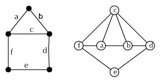
Menger’s theorem also generalizes in the obvious way to directed graphs, though we shall not give a statement or proof here.
4 Network Flows, Max-flow/Min-cut
And he thought of himself floating on his back down a river,
or striking out from one island to another, and he felt that
that was really the life for a Tigger.
The house at Pooh corner
A. A. Milne
A network is a digraph with weighted edges with two distinguished vertices, the source and the target . We assume that the weights (which we call capacities) are nonnegative. (Below we shall assume that weights are in fact rational – clearly we can approximate real weights to arbitrary precision. We shall investigate the issue of irrational capacities in the exercises.) An example is given in Figure 4. For a (directed) edge we denote by the initial, and by the terminal vertex of this edge.
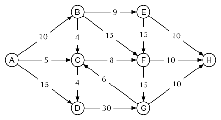
The reader might want to consider this as a network of roads with weights being the maximal capacity. (It is possible to have different capacities in different directions on the same road.) We want to transport vehicles from to (and implicitly ask how many we can transport through the network).
Note that we are looking for a steady state in a steady-state transport situation; that is we do not want to transport once, but forever, and ask for the transport capacity per time unit.
A flow is a function defined on the edges (indicating the number of units we transport along that edge) such that
-
•
(do not exceed capacity).
-
•
(No intermediate vertex can buffer capacity or create new flow. This is Kirchhoff’s law in Physics.)
The value of a flow is the net transport out of the source:
This definition might seem asymmetric in focusing on the source, however Lemma 4.1 will show that this is a somewhat arbitrary choice.
The question we ask thus is for the maximal value of a flow. The main tool for this is to consider the flow passing “by a point” in the network:
A cut in a network is a set of vertices such that , . We do not require the cut to be connected, though in practice it usually will be.
We note that the value of any flow is equal to the net flow out of a cut. (This implies that the value of a flow also is equal to the net transport into the target):
Lemma 4.1.
Let be a cut. We denote the edges crossing the cut by
Then for any flow we have that
Proof 4.2.
We prove the statement by induction on the number of vertices in . For we have that and the statement is the definition of the value of a flow.
Now suppose that , let and . By induction, the statement holds for .
We now consider the following disjoint sets of edges:
Any edge that starts at must be in or in , any edge ending at must be in or in . Kirchhoffs law thus gives us that
It is easily seen that , and that and . Therefore, using the previous expression to replace a difference of -sums by a difference of -sums:
The claim follows by induction.
We define the capacity of a cut as the sum of the capacity of the edges leaving the cut:
Lemma 4.1 thus implies that the value of any flow must be bounded by the capacity of any cut and thus (unsurprisingly) the maximal flow value is bounded by the minimum cut capacity – a chain is only as strong as its weakest link.
Similar to the dualities we considered before, equality is attained:
Theorem 37 (Max-Flow Min-Cut, integer version).
Suppose the capacity function in integer valued. Then the maximum value of a flow in a network is equal to the minimum capacity of a cut. Furthermore, there is a maximum flow that is integer valued.
Note 4.3.
If the capacity function is rational valued, we can simply scale with the lcm of the denominators and obtain an integer valued capacity function. In the case of irrational capacities, the theorem holds by a boring approximation argument.
Proof 4.4 (MengerMax-flow).
Given a directed network, replace every arc with integral weight by disjoint444Or edges with intermediate vertices to ensure disjointness directed edges.
Clearly, if one edge of a -fold multi-edge set is in a minimum separating set, the other edges have to be.
Thus the cardinality of a minimum edge-separating set is a minimum cut, while independent paths give a flow of . By the edge version of Menger’s theorem, the minimum cardinality of an edge-separating set equals the maximum number of independent edge paths, proving the theorem.
The existence of a maximum flow with integer values will follow from the following algorithm.
The algorithm of Ford and Fulkerson finds a maximal flow for a given network. It start with a valid flow (say for all edges) and then improves this flow if possible, using the following main step: {algo}[increase flow] Given a flow , return a flow with higher value, or show that no such flow exists.
-
1.
Let . \alginvar is a cut of vertices that can be supplied at higher rate from the source. . \alginvar is a set of edges that are not yet at capacity. . \alginvar is a set of edges whose flow should be reduced.
-
2.
If , go to step 6.
-
3.
If there is an edge with , set , . Go to step 2.
-
4.
If there is an edge with \alginvarThis is flow into which we could reduce, set , . Go to step 2.
-
5.
If neither of these two properties hold, terminate with a message that the flow is maximal.
-
6.
By tracing back how got added to , we construct an (undirected) path (the augmenting path) from to . Let
Increase the flow on by , reduce the flow on by . \alginvarThis satisfies Kirchhoffs law. Return the larger flow.
Proof 4.5.
We shall show termination in the case of integral capacities: Every time we adjust a flow, we may assume that the flow on one edge increases by an integral value. This can only happen a finite number of times.
We illustrate the algorithm in the example from above. Figure 5, a) shows some flow (in blue). The total flow is 24.
We start building the list of under-supplied vertices and mark edges on which to increase, respectively reduce the flow:
| Vertices | Increase | Reduce |
| s | ||
| B | sB | |
| A | AB | |
| D | AD | |
| t | DT |
We find an augmenting path sBADt (red in Figure b) and note that we can increase the flow by 2 (the limiting factor being edge sB) to a total of 26.
Starting again, we obtain (Figure c) the augmenting path sCFBAEt, on which we can increase the flow by 2 again, resulting is a flow of 28.
Finally we build the under-supplied cities as C,F,B and then cannot increase the set. Thus (Figure d), shaded) is a cut whose capacity of 28 is reached, proving that we have a maximal flow.
a)
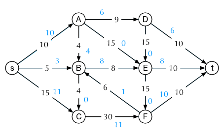 b)
b)
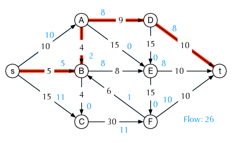
c)
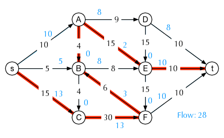 d)
d)
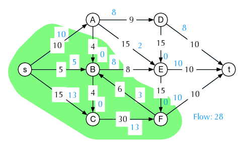
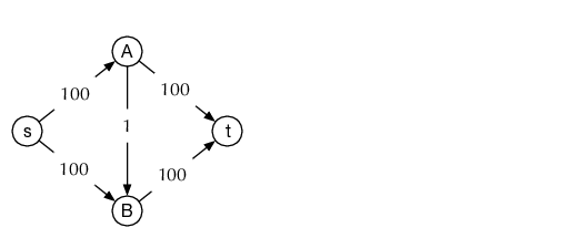
Note 4.6.
As given, the algorithm is not necessarily in polynomial time, as there might be a huge number of small incremental steps. Take the network in Figure 6. Starting with a flow of 0, we choose the augmenting path sABt on which we can increase the flow by 1. Next, we take the augmenting path sBAt, reducing the flow on AB to 0 again and have a total flow of 2. We can iterate this, increasing the flow by 1 each step until we get the maximum flow of 200.
Polynomial time in this algorithm however can be achieved by a more careful choice of the augmenting path (e.g. a shortest path, Edmonds-Karp algorithm), that analysis however is beyond the scope of these notes.
Note 4.7.
To close the circle, observe that the Max-flow/Min-cut theorem implies Dilworth’s theorem: Given a poset, we model it as a directed network with flow from bottom to top and arc capacity one. Thus all theorems mentioned in this section (and in fact a few more we have not mentioned) are in a sense mutually equivalent and form the fundamental theorem of discrete optimization.
1 Braess’ Paradox
On Earth Day this year, New York City’s Transportation Commissioner decided
to close 42d Street, which as every New Yorker knows is always congested.
”Many predicted it would be doomsday,” said the Commissioner […]
But to everyone’s surprise […]
Traffic flow actually improved when 42d Street was closed.
New York Times, 12/25/1990, p.38
Gina Kolata
From the time of Say and Ricardo the classical economists have taught that
supply creates its own demand
The General Theory of Employment, Interest, and Money
John Maynard Keynes
Often the question of maximal flow turns up not just for an existing network, but already at the stage of network design, aiming to maximize flow. Braess’ paradox shows that this can be very nonintuitive.
While we shall give a theoretical example, concrete instances of this effect have been observed in the real world in several cities (New York; Stuttgart, Germany; Winnipeg, Canada;…) when roads had been temporarily blocked because of building work, or after new roads were built. The interested reader might observe obvious implications to society and politics.
Suppose we have four cities, A, B, C, D with connecting roads as shown in figure 7, left. The reader may observe that this configuration is similar to the one in Note 4.6.
Cities A and B as well as C and D are connected by a minor road which easily clogs up. The driving time thus depends strongly on the number of cars, it is
with the number of drivers in thousands. An obstacle blocks direct connections from B to C.
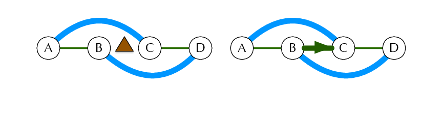
High capacity roads have been build to connect A and C, as well as B and D. While overall time is longer, the impact for extra cars is less. Driving time with thousand drivers on the road is
Assume 6000 drivers want to travel from to . A symmetry argument shows that half (3000) travel via and half via . Their individual travel time is . It is not hard to show that this is a stable equilibrium, i.e. no traveler can gain by changing their route. Furthermore, the system will settle in this equilibrium by itself, as long we assume drivers want to minimize their travel time and when starting their journey have perfect knowledge of how many cars are on each road.
Eventually, a new connection is built from B to C through the obstacle (right image). (For simplicity of the argument we shall assume that it is one-way, but that is not crucial for the paradox, but only simplifies analysis.) It has high capacity and is short, so travel time on this route is
We now have three possible routes from to : , , and . Again assuming perfect information, drivers will move towards a distribution in which travel time along all possible routes is equal. We claim that such an equilibruum exists with 2000 drivers each using , and . (This means that 4000 drivers are traveling AB and CD, respectively, 2000 travel BC.) This is because we have
Again, one can show that this is the only equilibruum, and that it is stable.
But this new optimal travel time is and thus more than before. Implications that this might have for society are left to the reader as an exercise.
References
Index
- algebra footnote 4
- antichain Definition 22
- Assignment problem §2
- augmenting path §2, item 6
- Bell number Definition 7
- binomial coefficient §1
- binomial formula §1
- bipartite §2
- capacities §4
- capacity §4
- cardinality §1
- Catalan number Definition 9
- cells §4
- chain Definition 12
- compositions §1
- convolution §1
- covers §2, §2
- cut §4
- derangement Definition 1, Definition 2
- derangements §5
- differentiation §1
- digraph Chapter 4
- distinguishable §4
- distributive §3
- Euler function §1
- exponential generating function §5
- extremal set theory §4
- Ferrers diagram §4
- flow §4
- functional equation §1
- geometric series §1
- greatest lower bound 1st item
- Hasse-diagram §2
- Hungarian Method §2
- incidence algebra §5
- independent §2, §3
- indistinguishable §4
- injective §2
- instable §1
- integer partition §4
- integration §1
- interval §5
- involution Definition 10
- join Definition 13
- join-irreducible Definition 15
- labeled §4
- lattice Definition 13
- least upper bound 2nd item
- line §2
- line graph §3
- linear extension Proposition 11
- lower factorial §1
- matching §2
- maximal §2
- meet Definition 13
- minimal §2
- Möbius function §5
- multisets §1
- network §4
- order ideal §3
- partially ordered set §2
- partition §4
- parts §4
- permutation §1
- poset §2
- power set §2
- Principle of Inclusion and Exclusion §1
- product rule §1
- source §4
- stable §1
- Stirling number of the second kind Definition 7
- sum rule §1
- summation rule §1
- surjective §2
- system of distinct representatives §1
- target §4
- term rank §2
- topological sorting §1
- total order §1
- unlabeled §4
- value of a flow §4
- vertex cover §2
- vertex path §3
- vertex separating §3
- Young diagram §4
- zeta function §5
Some Counting Sequences
Bell
OEIS A000110, page 7
Catalan
OEIS A000108, page 9
Derangements
OEIS A000166, page 5
Involutions
OEIS A000085, page 10
Fibonacci
OEIS A000045, page 2
Partitions
OEIS A000041, page LABEL:partdef