DISCRETA Manual

Anton Betten

1 What is DISCRETA ?

Welcome to DISCRETA. DISCRETA is a program for the construction of incidence structures, t-designs, with prescribed automorphism group. A t-design, or more precisely a t-(v,k,l) design for integers t, v, k and l, is a finite incidence structure, i.e. a finite set of points together with a set of subsets. More precisely, a t-design is a pair (P,B) with P a set of v points, and B a set of k-subsets of P. The set B has the property that whichever t-subset of P is chosen, there are exactly l sets in B containing the chosen set of t points. The sets in B are also called blocks. Hence for any t-subset of points we find exactly l blocks containing them.

The idea to construct such incidence structures is by means of a prescribed automorphism group. An automorphism is just a permutation of the set of points such that when applied to each of the blocks, the set of blocks as a whole is preserved. Here, when we say, we apply a permutation to a block, we mean that we apply the permutation to all point in the block. We then collect all the k points which we get and form a new block of size k out of these (we call this the image of the original block under the given permutation). Of course for a permutation to be an isomorphism, each image block must be contained in B since we required that the set of blocks as a whole stays invariant under that permutation. Now, the set of such automorphisms form a group w.r.t. composition. This means for elements a and b which are automorphisms, the composition ab is again an automorphism. Also, the inverses a^-1 are automorphisms. The identity mapping which takes each point to itself is trivially an automorphism. It serves as the identity element in the automorphism group.

Why do we do all this? Well, the construction of t-designs can be a hard task, in particular for certain parameter combinations. t-designs with large t are known to be notoriously hard to construct. At this point, Kramer and Mesner in 1975 introduced their method of constructing designs which are invariant under a group of automorphisms. The clue is that the construction of designs using a prescribed automorphism group becomes much easier the larger the group is. We do not give the details of this construction, but rather go back to DISCRETA and explain how to use this program for this method.

At this point, we see two basic steps in the construction of designs.

First, we have to fix a set of parameters t, v, k and l of the design we wish to construct. In addition, and rather more at the same time as fixing the parameters, we have to choose a group which shall serve as automorphism group of the design. Of course, the group should be a permutation group on v points, since our design will have v points. The group should have the right size for the problem, i.e. its order should somehow match the difficulty of the problem, since otherwise we may not be able to construct designs at all. Of course, it is a difficult task to choose the right group and often we have to try several possibilities. Let us denote the group we have chosen by G.
Secondly, we finally got to construct the designs which are invariant under the group G chosen in the first step. This is where the parameters t and k come into play (recall that we have chosen all parameters in the first step). We compute a matrix which is determined by the choice of the group and the choice of t and k (so far, the last parameter l is not yet considered). In honor of Kramer and Mesner's contribution, this matrix is called the Kramer Mesner matrix of the construction. Once the Kramer Mesner matrix is there, the last parameter l comes in and we form a diophantine system of equations with the Kramer Mesner matrix on the left, and a vector whose entries are all l on the right. The system has to be solved for another integer vector, but this time we are restricted to the integers zero and one. The solutions to this system are in one-to-one correspondence to the t-(v,kj,l) designs with prescribed automorphism group G. (i.e. all the designs which are invariant under G).

At this point, if we have found solutions in the second step, we can consider the construction problem of such designs solved. However, we will see that there is also the classification problem of such designs and we will come back to that problem at a later stage.

2 Step 1, we choose a group

As described previously, we have to choose parameters t, v, k and l as well as a permutation group G acting on v points. First of all, we have t < k < v positive integers. In order to be successfull, the design parameret set t-(v,k,l) must satisfy one combinatorial condition. This condition is on l in terms of the other three parameters. More precisely, there are two numbers, Dl and l_max, depending only on t, v and k, and l must be a multiple of Dl but less than l_max. Note that these conditions are only necessary conditions, in other words, we wouldn't find designs if the condition is violated. The conditions are not sufficient for the existence of designs. Note that the condition l not equal l_max just excludes the trivial designs, which consist of all k-subsets of the set of points, which are always t-designs, but at the same time are not very interesting (just because we know they exist for all t < k < v). A design parameter set which satisfies this condition is called admissible.

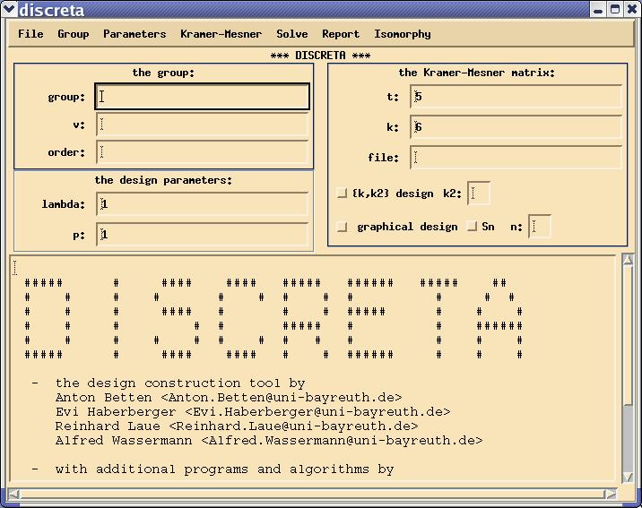
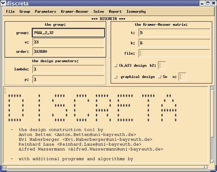
DISCRETA helps choosing l by computing Dl once t < k < v have been chosen. Let us have a look at the DISCRETA main window:

Suppose you plan to construct a 7-(33,8,l) design. Type 33 into the box for v, type 7 and 8 into the boxes for t and k, respectively. In addition, fill in a 1 into the box for l. Then go into the menu and choose lambda_i in the Parameters menu. The program will produce output in your terminal like this

The discreta_batch calc_lambda_ij 7 33 8 1
calc_lambda_ij t v k lambda
calc_delta_lambda(): v=33 t=7 k=8 lambda=1
t'=6 lambda'=27/2 delta_lambda=2
t'=5 lambda'=126/1 delta_lambda=2
t'=4 lambda'=1827/2 delta_lambda=2
t'=3 lambda'=5481/1 delta_lambda=2
t'=2 lambda'=56637/2 delta_lambda=2
t'=1 lambda'=129456/1 delta_lambda=2
t'=0 lambda'=534006/1 delta_lambda=2
warning: this parameter set is not admissible, lambda must be a multiple of 2 !

What has happened? Your input amounts to the parameters t-(v,k,1), i.e. with lambda = 1. DISCRETA computes the parameters of the design as an t' design for 0 less or equal t' less than t. The resulting poarameter sets t'-(v,k,lambda') should all be integral, and Delta lambda will be computed as the smallest natural number lambda such that all lambda' are integral. In this case, DISCRETA detects that lambda must be a multiple of Delta lambda, which is 2. Note that if you would have started with an admissible parameter set like 7-(33,8,10), the output would be

calc_lambda_ij t v k lambda
calc_delta_lambda(): v=33 t=7 k=8 lambda=1
t'=6 lambda'=27/2 delta_lambda=2
t'=5 lambda'=126/1 delta_lambda=2
t'=4 lambda'=1827/2 delta_lambda=2
t'=3 lambda'=5481/1 delta_lambda=2
t'=2 lambda'=56637/2 delta_lambda=2
t'=1 lambda'=129456/1 delta_lambda=2
t'=0 lambda'=534006/1 delta_lambda=2
 5340060  4045500  3034125  2251125  1650825  1195425  853875  600875
 1294560  1011375   783000   600300   455400   341550  253000       0
  283185   228375   182700   144900   113850    88550       0       0
   54810    45675    37800    31050    25300        0       0       0
    9135     7875     6750     5750        0        0       0       0
    1260     1125     1000        0        0        0       0       0
     135      125        0        0        0        0       0       0
      10        0        0        0        0        0       0       0

This time, DISCRETA does not complain, and you find the parameter sets t'-(v,k,lambda') for 0 less or equal t' less than 7. Also, DISCRETA lists some more parameters which are tabulated in form of a matrix. These are the lambdai,j for i+j less or equal t (and zeroes elsewhere). The value of lambdai,j is the number of blocks in the design which contain a given set of i points and which are disjoint from another given set of j points, provided that the two sets are disjoint and that i + j is at most t.

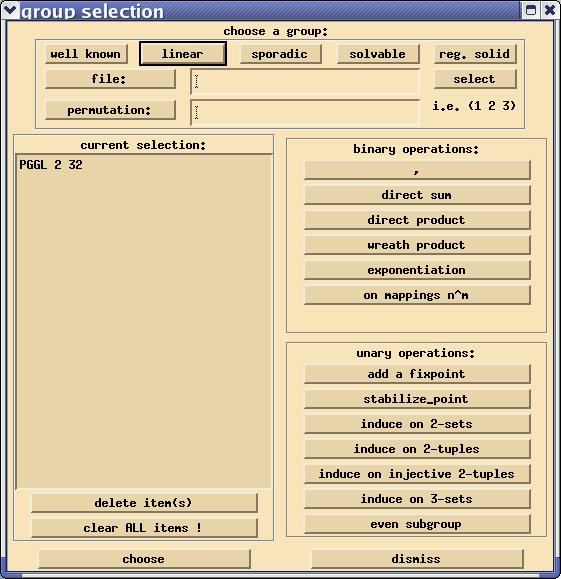
Let us now describe how to choose a group, by which we mean a group together with a permutation representation. First, go into the Group menu and choose Choose prescribed automorphism group. The main group selection dialog will appear:

This dialog is for composing a permutation group. A permutation group is constructed in a step-by-step fashion, building up a recipe, which is then executed by DISCRETA. The recipe can be very simple, i.e. just one line, or it can be lengthy and complicated. It is important to understand that DISCRETA does not actually construct the group until the recipe is complete. Each step in the recipe is either the choice of a group or a modification of something which is already there. On the left side of the dialogue, a listbox will show the construction steps defined so far. The other buttons are for selecting either groups (permutation groups) or modification commands. The buttons delete item(s) and clear ALL items ! below the listbox are for removing either the last entry or all entries which are shown in the listbox. Below are two buttons labelled choose and dismiss. The choose butten at the bottom constructs the group by executing the recipe, while the dismiss button just leaves the dialogue without constructing any group. Note that only by pressing the choose button, the actual construction process for the permutation group is started. If successfull, the group, v and order fields in the main window will show the name of the group, the degree as a permutation group, and the group order, respectively. If unsuccessfull, some error messages will appear in the terminal window, and you may start over with the group selection dialogue again.

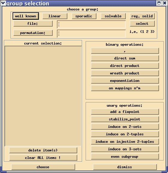
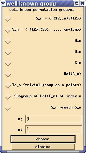
Let us describe now how to construct a group. Most impartant are the five buttons in the top row, labelled well known, linear, sporadic, solvable and reg. solid. Each of these opens another dialogue, where certain pre-defined permutation groups can be chosen. Consider the first one well known. After clicking on the button, the dialogue

appears. In this dialogue, built in groups like the symmetric group (S_n), the alternating group (A_n), cyclic groups (C_n), Dihedral groups (D_n) and others can be constructed. The parameters n and m (if necessary) can be specified in the text fields below. Pressing choose does not actually construct the group but just adds another entry to the group selection listbox mentioned above. The other groups in this dialogue are the holomorph of a cyclic group, i.e. the cyclic group C_n extended by the multiplications with elements which are prime to n. This group is of order n ·j(n), where j is the Euler function. The trivial group which consists of just one element, the identity, is sometimes needed. The button Id_n (trivial group on n points) allows to construct this group. The next button allows to construct a subgroup of the holomorph of the cyclic group C_n. Here, the integer m is the index in the holomorph. Also, there is a button which constructs the wreath product S_n \wr S_m in the permutation representation on nm points.

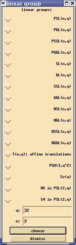
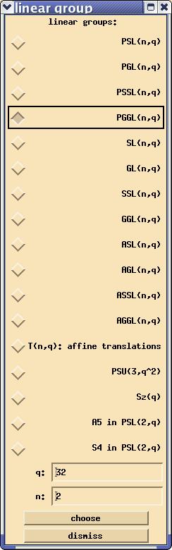
Let us go back to the group selection dialogue. The next button entitled linear opens the dialogue

where various linear groups can be chosen (it should be clear how to chose one of those groups: type in the parameters n and q and press the button of the correspoinding group). One word concerning notation. The linear group PGL(n,q) consists of all the projective linear mappings induced by non-singular n by n matrices over the field GF(q) with q elements (q is a power of a prime). PSL(n,q) is the subgroup which is induced my non-singular n by n matrices over the field GF(q) with determinant 1. If q is not prime, i.e. if q = p^e with p prime and e an integer greater than one then the map F: x goes to x^p is an automorphism of the field GF(q) which is the identity map on the elements of GF(p). The order of F is e. We can consider semilinear maps which consist of a linear map together with a suitable power of F where F acts component-wise on the vectors in GF(q)ⁿ. We may consider this action projectively, i.e. acting in the one-dimensional subspaces of the vector space. What we get is a group PGGL(n,q) (read "P Gamma L"), which is the extension of PGL(n,q) by the mappings induced from F acting component-wise on the vectors. We may consider the subgroup PSSL(n,q) (read "P Sigma L") which consist of all semilinear maps whose linear part stems from a matrix of determinant one.

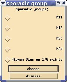
Back in group selection, the next button entitled sporadic opens the dialogue

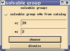
where various Mathieu groups or the Higman Sims group can be chosen.

The fourth button in group selection, entitled solvable opens the dialogue

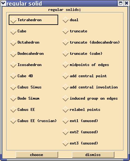
where solvable groups can be chosen from a catalogue of solvable groups of smnall order. These functions are currently inactive.

The last button in group selection, entitled reg. solid opens the dialogue

for choosing symmetry groups of platonic and archimedian solids. Remember that we have said that we a specifying a permutation group? The point is that a permutation group acts on on `something'. This something will be a set of points labelled 1,..., d where d is the degree. Now here is the important point: while previously we were acting on abstract integers, now we consider also the object itself, on which we act as a permutation group. By object we mean a solid in Euklidean space, for example a Platonic solid or an Archimedian solid, but we are not restricted to only those. We then act on the vertices of this solid as a symmetry group, i.e. we always map the solid to itself. Interestingly, not only do we construct the symmetry group. We also construct the object itself, together with a labelling of its vertices and the embedding of the symmetry group as a permutation group on those vertices. In a moment, we will be able to see the object in a three dimensional representation.

After choosing a group G by specifying a recipe in the group selection dialogue, and after pressing the button choose and successfully constructing the group, we will see the name of the group, the permutation degree, and the group order in the three fields group, v and order in the DISCRETA main window. From now on, G is fixed.

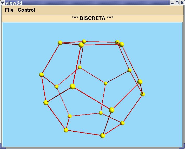
In case that we have chosen a symmetry group of an Euklidean object, we may decide to actually see this object itself. For this, we go into the Group menu again and choose show solid. Another window opens up, displaying the object in 3D-space, for instance as

It is useful to know that this window actually stems from another program, called view3d, which is called automatically. The view3d program is useful for visualizing the object in 3D space. We are able to rotate the object by mouse drag. We stop a rotating object by a single click. We can zoom in and out of the object. The actual numbering of vertices is not visible in the 3D representation. But we may choose to check the menu entry show labels and then decide to print the obejct, which results in a 2D projection of the object, printed into a tex document. The actual graphic is translated into a metapost graphic and translated automatically into eps format by that program. The files are created in the current directory. Feel free to take the graphic and include it in your other tex documents. Note that for some reason the eps files have the extension dot one (.1), but they are really eps files.

Any time you have defined a group, you may choose to investigate its subgroup lattice. For this, go into the Group menu again and choose calc subgroup lattice: w.r.t. inner automorphisms. You may wish to invoke this funtion only for groups of moderate size (i.e. at most a few thousand elements), since otherwise the computation becomes too time and memory intense. Assume we still have the group of the Dodecahedron, which is isomorphic to A₅. Then coosing the button results in a small computation, which can be traced in the terminal window. The final output looks like

{1,3,3,1,1} 9
{1,31,21,5,1} 59
computation of subgroup lattice finished.

The two rows of numbers correspond to the number of conjugacy classes of subgroups (first row) and the number of subgroups (second row) in each layer of the subgroup lattice. The layers are determined by the number of prime factors (including multiplicities), dividing the order of a subgroup. the layers are listed in brackets, going up from layer 0 (the trivial subgroup) to the highest layer (the group itself). Afterwards, the total number is given.

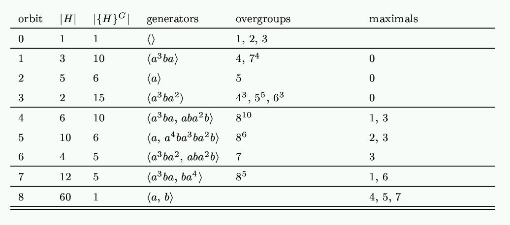
In order to actually see the subgroup lattice, go into the Group menu again and choose show subgroup lattice, Burnside matrix. A latex document will be prepared and translated autopmatically. If you browse this document, you may find on the second page a graphical display of the subgroup lattice. In case of the group of the Dodecahedron, A₅, we obtain:

(You may have to change the orientation of the view in the postscript display program to get the picture upside down.) If you browse to the following page, you should get a description of the subgroups by conjugacy classes. In the case of A₅ you will see ./sgl_a5_labels.jpg

The first column lists the number of the orbit, i.e. the conjugacy class of subgroups. This number corresponds to the number shown in the graphical dispolay of the lattice. For H one group of the conjugacy class, the following columns list the order of the group H as well as the length of the conjugacy class, i.e. the order of H^G. The generators column lists H as generated by elements in H. These elements are written as words in the generators of G, so it is critical to know the generators for G. The following two columns list the types of overgroups and maximal subgroups of H. An entry like 4³,5⁵,6³ in the overgroup column (in line 3) means that H of class 3 has 3 overgroups of class 4, 5 overgroups of class 5 and 3 overgroups of class 6.

3 Step 2, we construct a design

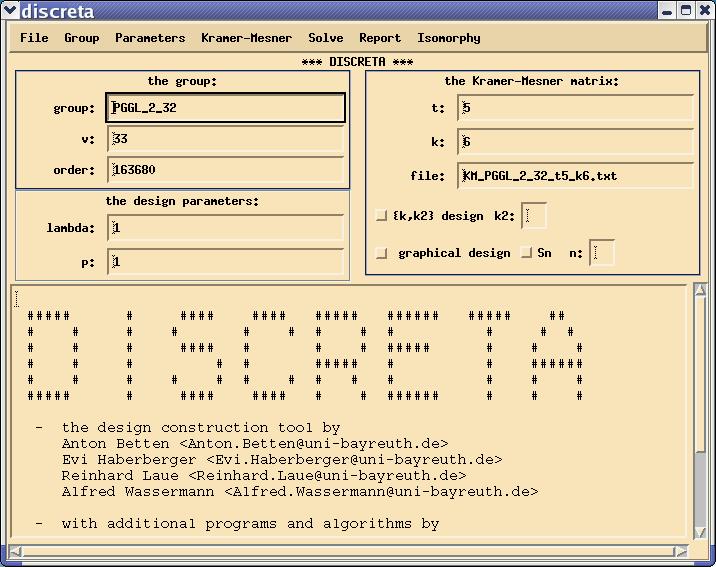
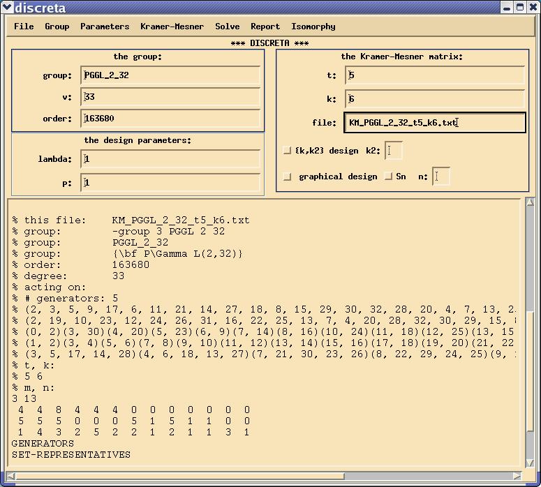
At the beginning of Step 1, we chose the design parameters t-(v,k,lambda). Indeed, the parameter v turned out to be the degree of the permutation group G we have chosen to prescribe. So far, the other three parameters did not come in, but this will change in a minute. In order to construct a design which is invariant under G we apply the method of Kramer and Mesner which allows to describe such designs as 0/1 solutions of certain integral systems of equations. The coefficient matrix of this system has already been introduced as the Kramer Mesner matrix. This matrix depends on G and on the parameters t and k, and hence we denote it as Mt,k^G. The rows are indexed by the orbits of G on t-subsets, whereas the columns are indexed by the orbits of G on k-subsets (of 1,...d, of course). The matrix entry corresponding to a t-orbit T^G and a k-orbit K^G is the number of elements K' in the orbit K^G which contain T. In order to compute Mt,k^G, we first specify G, which we already did in Step 1. We now put in the values of t and k into the corresponding text fields in the main window. After that, we choose compute Kramer Mesner matrix from the Kramer-Mesner menu to actually compute the matrix Mt,k^G. The actual computation produces some output in the text window. The orbits of G on sets of size at most k are computed by an induction on the size of the sets. In the end, a file is created containing all the data from the computation. The filename starts with "KM_", then comes the name of the group, and after that the values of t and k in the format t`value of t'_k`value of k'. The extension is ".txt". We call this the KM-file. Its name appears in the file text field in the main window. We may want top have a look into that file. For this, we choose show matrix in the Kramer-Mesner menu. We may have to scroll within the larg text field in the bottom half of the DISCRETA window, to find the actual contents of the file. We are now ready to construct the designs. We choose lambda and enter the value into the lambda text field. Then we choose LLL in the Solve menu. We get information about the existence or nonexistens of solutions in the terminal window. Note that DISCRETA always trues to compute the complete set of solutions, i.e. the number which is given (if the program terminates successfully) is the exact number of designs with that prescribed automorphism group. Note, however, that this does not give the number of isomorphism types of designs. That number is to be determined later. In order to be able to work with these solutions later on, we choose get solutions from solver in the Solver menu, which copies the solution vectors into the KM-file.

Example: Assume we want to construct designs invariant under PGGL(2,32). We go into the group selection dialog and from there into the dialog for linear groups. We fill in n = 2 and q = 32 and click on PGGL:

Then, we click choose and recognize that the listbox in the group selection dialog contains one entry corresponding to our choice (we also click on dismiss in the linear dialog to get rid of that dialog). The group selection dialog now looks like: ./group_selection3.jpg

The next step is to click choose (and afterwards dismiss) in the group selection dialog. This finally creates the group we specified, and we can check the label of the group, the degree and the order in the DISCRETA main window, which should now look like: ./main3.jpg

Note that if some previous calculation of DISCRETA has take place then there might be a valid file name in the file text filed. We can ignore this for now. We now have to decide about the parameters t and k of the design. Let us choose t = 5 and k = 6, which are actually preselected by DISCRETA. If we would choose different values, we would have to fill in the textfields t and k, of course. After choosing the compute Kramer Mesner matrix menu entry, the computation start. After a while, and after a considerable amount of output to the terminal, the computation finishes. The main window looks like ./main4.jpg

(Note the file name "KM_PGGL_2_32_t5_k6.txt" in the file text field). We choose show matrix in the Kramer Mesner menu, and after a little scrolling, the main window could look like ./main5.jpg

We note that the header of the file shows basic information about the parameters of the design, as well as on the group. We can find generators for the group as permutations. After that, we see the Kramer Mesner matrix, preceeded by information about its size. This part is

% m, n:
3 13
 4  4  8  4  4  4  0  0  0  0  0  0  0
 5  5  5  0  0  0  5  1  5  1  1  0  0
 1  4  3  2  5  2  2  1  2  1  1  3  1

We know choose lambda = 12 (If we don't know what to choose we can ask the lambda_i function in the Parameters menu. in this case, we get a value of Dl of 4, and after unsuccessfully trying 4 and 8, the next candidate is lambda = 12.) After that, we choose LLL in the Solve menu, which starts the actual solving process for designs. After a short while, we see some output in the terminal window. The output finishes by telling us about the number of solutions which could be found:

0010100110100 L = 12
0010101001100 L = 12
0010100011100 L = 12
0010101101000 L = 12
0010100111000 L = 12
Prune_cs: 103
Prune_only_zeros: 4 of 106
Prune_hoelder: 0 of 102
Prune_N: 1
Fincke-Pohst: 2
Loops: 265
Total number of solutions: 54

calling ...
tail -10 lll.log >lll.log.1
finished !

In this case we have 54 solutions, all of which are displayed as 0/1 vectors (we show only the last 5 of them here). We finally choose get solutions from solver in the Solver menu to copy the solution vectors into the KM-file.

File translated from T_EX by T_TH, version 3.12.
On 1 Jul 2003, 21:23.